Comparison of MPPT Strategies in Battery Charging of Photovoltaic Systems João H. de Oliveira1, Luan P. Carlette3, Allan F. Cupertino2,3, Victor F. Mendes1 , Wallace do C. Boaventura1 and Heverton A. Pereira1,3 1
Graduate Program in Electrical Engineering Federal University of Minas Gerais Av. Antônio Carlos 6627, 31270-901 Belo Horizonte, MG, Brazil
[email protected],
[email protected]
Gerência de Especialistas em Sistemas Elétricos de Potência Universidade Federal de Viçosa Av. P. H. Rolfs s/nº, 36570-000 Viçosa, MG, Brazil
[email protected],
[email protected]
Index Terms—MPPT algorithm, buck converter, battery, standalone.
INTRODUCTION
One of the major energy challenges in the world is ensuring access to clean and sustainable energy. Solar energy has been gaining more widespread concern because of its advantages of clean and free pollution as well as inexhaustible use. Photovoltaic (PV) arrays are used in many applications such as water pumping, battery charging, hybrid vehicles, and grid connected PV systems. In this context, solar PV systems have growth considerably. According to a survey released recently by European Photovoltaic Industry Association (EPIA), in 2013 the installed capacity of PV modules reached a value around 132 GW worldwide [1]. A photovoltaic generator is a current source strongly dependent on climatic conditions (solar irradiance, temperature, wind speed, etc.). Thus, it is necessary to extract as much power as possible from a solar panel. For a given value of irradiance
and temperature there is a point which the maximum power is obtained. For this reason, in PV systems there is a maximum power point tracker (MPPT) which can optimize the system controlling the panel voltage to the maximum power point. The MPPT acts in order to force the operating point of PV modules on their peak power. The MPPT algorithm work in two different forms: calculating directly the duty cycle of the power converter, similarly to an open loop control, or calculating the maximum power point voltage which is reference for a voltage closed loop control. The second method is preferable because it reduces losses and the stress of the converter by limiting the bandwidth of the duty cycle [2]. Several MPPT algorithms have been proposed in the literature. This work studies three strategies: perturbation and observation (P&O) [3], dP-P&O [4] and Modified P&O (MP&O) [5]. Simulations were performed to evaluate the instantaneous and dynamic efficiency of three MPPT algorithms during changes in solar irradiance. Duty Cycle 0.1 50
0.2
0.3
0.4
0.5
0.6
0.7
0.8
0.9
1 0.81
PV power PV power considering efficiency
45
0.805 Converter efficiency
40 0.8 35 0.795
30 25
0.79
20
Efficiency
Abstract— In photovoltaic standalone systems it is crucial to absorb most of the available energy. Thus, in order to extract the maximum power of a solar panel for a given set of climatic conditions, it is used maximum power point tracker (MPPT). The MPPT consists in a power converter which controls the solar panel voltage. In this context, this work compares the instantaneous and dynamic efficiency of three MPPT algorithms proposed in literature: perturb and observe, dP - perturb and observe and modified perturb and observe used in a photovoltaic standalone systems. The system analyzed is composted by a 48 W solar panel, a battery of 60 Ah and a charger based on a buck converter. During solar irradiance variations the algorithms presented different instantaneous efficiencies, what can produce reduction in energy absorbed during cloudy days.
I.
Departamento de Engenharia de Materiais Centro Federal de Educação Tecnológica de Minas Gerais Av. Amazonas 5253, 30421-169 Belo Horizonte, MG, Brazil
[email protected]
Power (W)
3
2
0.785
15 0.78 10 0.775
5 0
0
5
10
15
20
0.77 25
Voltage (V)
Figure 1 – Solar panel PV curve considering the buck converter efficiency. This work is supported by the Brazilian agencies CAPES, FAPEMIG and CNPQ.
Rechargeable batteries are widely used in standalone photovoltaic systems to store energy. The most common type used is the sealed maintenance free lead acid battery [6]. A battery charging controller is essential to increase the lifetime of the battery [6], [7]. In this paper, the battery charging system is implemented with a Buck converter. Figure 1 shows how the maximum power point of a PV panel is limited by the efficiency of the buck converter. This efficiency is function of duty cycle, which is controlled to keep the voltage on the battery. II.
MPPT ALGORITHMS
One of the most frequently used MPPT methods is the Perturb and Observe (P&O) algorithm, due to its low complexity and the low computational power it needs. However, if the change in the insolation intensity causes bigger change in power than the one caused by the increment in the voltage, the MPPT can misinterpret the change in the power as an effect of its own action [4].
B. dP-P&O method The dP-P&O method is an improvement of the classical P&O in the sense that it can prevent itself from tracking in the wrong direction during rapidly changing in the solar irradiance. This method performs an additional measurement of power in the middle of the MPPT sampling period without any perturbation, as can be seen in Figure 3. Considering de power rate is constant over one sample period, which is a good approximation in most of the cases, the change in power between and reflects only the change due to the environmental changes, since no action has been made by the MPPT. [4].
Hence, variations of P&O are proposed in literature to solve problems caused by the rapidly changing in irradiance. The explanation of the methods discussed in this work is detailed in the following sections. A. Perturbation and observe – P&O Perturbation and Observation (P&O) algorithm is presented in [8]. This method have been widely used due to its low complexity and origins many other algorithms as Modified P&O, Hill Climbing and Modified Hill Climbing [9]. P&O algorithm periodically increments or decrements the solar array voltage and compares the output power with the previous value. If the delivered power increased, the perturbation will continue in the same direction in the next cycle, otherwise the perturbation direction changes. This means a perturbation in the array terminal voltage in each and every cycle. When the MPP is reached, P&O algorithm will oscillate around it [10]. Figure 2 shows the flow chart of the P&O method.
Figure 2 – P&O method flow chart.
Figure 3 – Measurement of the power between two MPPT sampling instances [4].
C. Modified P&O The Modified P&O (MP&O) method decouples the PV power fluctuations caused by hill-climbing process from those caused by irradiance changing [11]. This method adds a process to estimate the irradiance change throughout perturbation to measure the amount of energy change caused by changing atmospheric conditions, and then compensates it for the next process of perturbation [5]. Figure 4 shows the flow chart of the Modified P&O method.
Figure 4 –Modified P&O method flow chart.
There are two operation modes named: Mode 1 for estimate process and Mode 2 for perturb process. Mode 1 measures the energy variation due to the change in voltage and atmospheric changes and maintains constant voltage PV to the next control period. Mode 2 measures the change in power and determines the new strain PV based on present and previous variations of energy [5]. D. Instantaneous and dynamic MPP-tracking efficiency Measuring the efficiency along the simulation gives much more information about the MMPT algorithms performances than the overall efficiency alone. Hence, the instantaneous and dynamic efficiency are important tools to compare the MPPT’s behavior. At locations, where there are often variable cloudy conditions, the dynamic MPPT behavior has to be considered. Inverters with a fast MPP-tracker have a somewhat higher energy yield under quickly changing irradiance than devices with a slow MPPT [12]. Thus, dynamic MPPT efficiency η
The simplified PV model is represented by a voltage source and a resistance [10], [13]. This simplification is used in the buck converter modeling linearization around the MPP. In [10] and [14] linearization is proved stable for a wide range of irradiance values. Figure 7 presents the IxV curve of a SM48KSM Kyocera panel and the linearization around the MPP for the nominal conditions. In this case, V = 37.05 V and R = 7.15 Ω. The parameters of the PV used for simulations are presented in Table 1. TABLE 1.
Parameters of the SM48KSM.
Parameter Maximum Power Maximum Power Voltage Maximum Power Current Open Vircuit Voltage Short Circuit Current Temperature Coefficient of Temperature Coefficient of
can be defined
Value 48 18.6 2.59 22.1 2.89 −0.07 / 0.00166 /
as 3.5 _
[%] = 100
η
(1)
_
where
η
[%] = 100
_
.
(2)
2.5
Current (A)
is the output power measured in the panel and _ is the maximum power of the panel available. _ The instantaneous efficiency is:
I x V curve Linearization
3
2 1.5
_
1
III.
BUCK CONVERTER
A. Modeling Figure 5 shows a PV system connected to a DC/DC converter, which is used to charge a battery. The output power of the PV array is controlled by the converter [10]. This work uses the buck converter, shown in Figure 6.
0.5 0 0
5
Figure 7 -
10 15 Voltage (V)
20
25
curve of the panel and its linearization around the MPP.
The state space equations of the converter are 〈 ̇〉 = +
Figure 5 - Scheme of a battery charger.
+ .( − ) .〈 〉 + .( − ) .〈 〉
(3)
where: In PV applications, the voltage control is preferable because the maximum power voltage of the panel is approximately constant over a wide range of solar irradiance changes [2]. The capacitor at the input of the converter reduces the input voltage ripple and filters the discontinuity in the input current.
1 ⎡− ⎤ ⎤ ⎥; ⎢ ⎥; = 1 ⎥ ⎢−1 − 1 ⎥ − . . ⎦ ⎣ ⎦ 1 1 ⎡ 0 − ⎤ − ⎤ ⎥; ⎥; ̇ = =⎢ 1 ⎢ 0 ⎥ 0 ⎥ ⎦ ⎣ . ⎦
⎡− =⎢ ⎢ 0 ⎣
0
⎡ 0 =⎢ 1 ⎢ ⎣ . = Figure 6 - Topology of the buck converter.
;
=
;
;
< X > represents the average value of the variable X. represents the average value of the duty cycle.
= + 〈 〉= + 〈 〉= +
(4)
Substituting (4) and (3) through algebraic manipulations, the result is:
1100 Profile 1 Profile 2
1000 900
Solar Radiation (W/m²)
Equation (3) is nonlinear because it involves multiplication of time-varying variables. Therefore, it is necessary to linearize the model. In [15] was proposed a methodology based on smallsignal model. The first step of this method is generating a small disturbance in steady state and verifying what happens to the system. Then,
800 700 600 500 400 300 200 100 0
̂
=
(5)
The transfer function relating the input voltage to the duty
( )=
( )=
( ) ( )
,
(6)
The complete structure of the battery charger is presented in Figure 8. The MPPT algorithm calculates the duty cycle of the converter.
0.1
0.15
0.2 0.25 Time (s)
0.3
Parameter Nominal Voltage Nominal Capacity Initial Stage of Charge Maximum Capacity Fully Charged Voltage Fully Discharged Voltage Nominal Discharge Current Internal Resistance
The performance of a 48 W battery charger based on buck converter was simulated using Matlab/Simulink software. Firstly, the performances of the MPPT algorithms were compared during variations in the incident solar irradiance according to the profiles presented in Figure 9, which slant and duration of the ramps are based in tests conducted in [12] . The parameters of the battery are shown in Table 2 and the parameters of the converter used in this simulation are in Table 3. The irradiance profiles used changes fast and, for this reason, it was considered that the temperature of the PV panel is constant along the simulation.
Value 12 6 ℎ 20 % 7 ℎ 14.14 8.00 6.25 0.018 Ω
Parameters of the converter.
Parameter Inductor – Capacitor in Panel – Output Voltage – Frequency Switching – Inductor Resistance –
IV. SIMULATIONS
0.4
Parameters of the battery (Nickel-Metal-Hydride).
TABLE 3.
Figure 8 - Battery charger with MPPT.
0.35
Figure 9 - Irradiance profiles used in the simulations. TABLE 2.
is:
0.05
Value 1.0 100 12 12 1Ω
V. RESULTS AND DISCUSSION A. Comparison of algorithms 1) 10-50% Irradiance ramp The first result is the PV power shown in Figure 10. In this figure curves for dP-P&O and MP&O are overlapping most of the time. P&O did not reach the MPP during the ramp and took at least 0.03s more to reach the MPP in comparison to the other two methods. The oscillations presented in P&O are caused by the limitation of this method to track right direction due to the rapid variation of irradiance. The P&O presents difficulty in tracking the value of the maximum power voltage, especially during the first ramp, right after 0.05s, as shown in Figure 11. PV current also features larger ripple in P&O due to the difficulty of tracking the right direction. The MP&O method presents a similar behavior to the dP-P&O, as shown in Figure 12.
50
25 dP-P&O P&O MP&O
40
15
Power (W)
Power (W)
20
10
30
20
10
5
0
dP-P&O P&O MP&O
0 0
0.05
0.1
0.15
0.2 Time (s)
0.25
0.3
0.35
0.4
Figure 10 – Behavior of the PV power for the studied algorithms for irradiance profile 1.
0
0.05
0.1
0.15
0.2 Time (s)
0.25
0.3
0.35
0.4
Figure 13 - Behavior of the PV power for the studied algorithms for irradiance profile 2.
25 dP-P&O P&O MP&O
25 dP-P&O P&O MP&O
Voltage (V)
20
Voltage (V)
20
15
15
10
0
0.05
0.1
0.15
0.2 Time (s)
0.25
0.3
0.35
0.4
10
Figure 11 – PV voltage for the studied algorithms for irradiance profile 1.
0
0.05
0.1
0.15
0.2 Time (s)
0.25
0.3
0.35
0.4
Figure 14 - PV voltage for the studied algorithms for irradiance profile 2.
1.5
3
dP-P&O P&O MP&O
dP-P&O P&O MP&O
2.5
1
Current (A)
Current (A)
2
0.5
1.5 1
0.5 0
0
0.05
0.1
0.15
0.2 Time (s)
0.25
0.3
0.35
0.4
0
0
0.05
0.1
0.15
0.2 Time (s)
0.25
0.3
0.35
0.4
Figure 12 – PV current for the studied algorithms for irradiance profile 1.
Figure 15 - PV current for the studied algorithms for irradiance profile 2.
2) 30-100% Irradiance ramp Figure 13 shows the PV power for the second irradiance profile. During variations of the incident solar irradiance dPP&O and MP&O method again showed a very similar behavior, but this time even P&O followed the shape of the curve, presenting more ripple in the second ramp when irradiance decreases to 30%.
B. Dynamic and Instantaneous Efficiency Table 4 indicates the dynamic efficiency for the three studied algorithms. Although the performances of all the three MPPT strategies are similar, dP-P&O has a better performance. The differences between the algorithms decrease to less than 1% for irradiance profile 2.
Figure 14 shows that the voltage is more stable for both three methods when responding for this irradiance profile. Figure 15 also shows a coincident shape, but P&O presents more ripple.
Analyzing Figure 16 it is possible to see the instantaneous efficiency of each algorithm for irradiance profile 1. A lot of variations in efficiency can be noticed especially during the ramps, being dP-P&O the most stable. For irradiance profile 2 all the algorithms perform better, dP-P&O is even more stable and MP&O and P&O have a similar behavior, as can be seen in Figure 17. TABLE 4 gives overall information about the
MPPT’s performance but Figure 16 e Figure 17 give more detailed information of how each MPPT behave during the simulation. TABLE 4. Dynamic efficiencies for both irradiance profiles.
Efficiency for Profile 1 (%) 96.4 96.0 98.9
P&O MP&O dP-P&O
Efficiency for Profile 2 (%) 98.7 98.7 99.4 600
100 500
Efficiency[%]
400 350
60
dP-P&O P&O MP&O Radiation
40
300 250 200
Irradiance [W/m2]
450
80
150 20
0
100
0
0.05
0.1
0.15
0.2 Time [s]
0.25
0.3
0.35
0 0.4
Figure 16 – Instantaneous efficiency for the three studied algorithms for irradiance profile 1
100
1000
dP-P&O P&O MP&O Radiation
50
600 500 400
Irradiance [W/m2]
Efficiency[%]
800
200
0
0
0.05
0.1
0.15
0.2 Time [s]
0.25
0.3
0.35
0 0.4
Figure 17 - Instantaneous efficiency for the three studied algorithms for irradiance profile 2
VI.
CONCLUSION
In standalone photovoltaic systems it is extremely important to guarantee the maximum efficiency considering the photovoltaic panels are the only energy source to charge the batteries and supply the loads. This paper presents a comparison of three MPPT algorithms. The dP-P&O presents the fastest response during irradiance variations due to the fact it tracks correctly the MPP direction. MP&O appears as a good solution to eliminate the problem of irradiance variation. Although the algorithms have a similar overall behavior, their performance differs more for low irradiance values and for irradiance ramps when measuring the instantaneous efficiency. Researchers are working on a prototype to test and compare the algorithms using real data.
REFERENCES [1] EPIA, "Global Market Outlook For Photovoltaics," 2014-2018. [2] M. G. Villalva, J. R. Gazoli and E. R. Filho, "Analysis and simulation of the P&O MPPT algorithm using a linearized photovoltaic array model.," in Proc. 2009 Brazilian Power Electronics Conference. [3] K. H. Hussein, . I. Muta, T. Hoshino and M. Osakada, "Maximum photovoltaic power tracking: an algorithm for rapidly changing atmospheric conditions," IEE Proceedings Generation, Transmission and Distribution, vol. 142, no. 1, pp. 59 - 64, 1995. [4] D. Sera, T. Kerekes, R. Teodorescu and F. Blaabjerg, "Improved MPPT method for rapidly changing enviromental conditions," in Proc. 2006 IEEE International Symposium on Industrial Electronics. [5] B. W. a. R. C. C. Liu, "Advanced Algorithm for MPPT control of Photovoltaic Systems," in Proc. 2004 Canadian Solar Buildings Conference. [6] B. Sree Manju, R. Ramaprabha and D. B. L. Mathur, "Modelling and Control of Standalone Solar Photovoltaic Charging System," in Proc. 2011 International Conference on Emerging Trends in Electrical and Computer Technology. [7] D. Ananth, "Performance evaluation of a solar photovoltaic system using maximum power tracking algorithm with battery backup," in Proc. 2012 IEEE PES Transmission and Distribution Conference and Exposition. [8] P. Midya, P. Krein, R. Turnbull, R. Reppa and J. Kimball, "Dynamic Maximum Power Point Tracker for Photovoltaic Applications," in Proc. 1996 Power Electronics Specialists Conference. [9] T. Esram and P. L. Chapman, "Comparison of photovoltaic array maximum power point tracking techniques," IEEE Transactions on Energy Conversion, vol. 22, no. 2, pp. 439449, 2007. [10] M. R. D.P. Hohm, "Comparative Study of Maximum Power Point Tracking Algorithms," Progress in Photovoltaics: Research and Applications, vol. 11, pp. 47-62, 2003. [11] H. Haeberlin and P. Schaerf , "New Procedure for Measuring Dynamic MPP-Tracking Efficiency at Grid-Connect PV Inverters," in Proc. 24th European Photovoltaic Solar Energy Conference, 2009. [12] M. G. Villalva, "Conversor Eletrônico de Potência Trifásico para Sistema Fotovoltaico Conectado à Rede Elétrica," Campinas, 2010. [13] A. F. Cupertino, J. T. Resende, H. A. Pereira and S. I. Seleme Júnior, "A Grid-Connected Photovoltaic System with a Maximum Power Point Tracker using Passivity-Based Control applied in a Boost Converter," in Proc. 2012 IEEE/IAS International Conference on Industrial Applications. [14] M. G. Villalva, J. R. Gazoli and E. Ruppert Filho, "Comprehensive Approach to Modeling and Simulation of Photovoltaic Arrays," IEEE Transactions on Power Electronics, vol. 24, no. 5, pp. 1198-1208, May 2009. [15] R. W. ERICKSON and D. MAKSIMOVIC', Fundamentals of Power Eletronics, New York: Klumer Academic Publishers, 2004.