Fluctuation and Noise Letters Vol. 7, No. 3 (2007) L273–L287 c World Scientific Publishing Company

Community dynamics in social networks

Gergely Palla Statistical and Biophysical Research Group of HAS, E¨ otv¨ os University, 1117 P´ azm´ any P´ eter s´ et´ any 1/A, Budapest, Hungary [email protected] Albert-L´ aszl´ o Barab´ asi Dept. of Physics, University of Notre Dame, IN 46566, USA [email protected] Tam´ as Vicsek Statistical and Biophysical Research Group of HAS, E¨ otv¨ os University, 1117 P´ azm´ any P´ eter s´ et´ any 1/A, Budapest, Hungary; Dept. of Biological Physics, E¨ otv¨ os University, 1117 P´ azm´ any P´ eter s´ et´ any 1/A, Budapest, Hungary [email protected] Received (10 July 2007) Revised (16 July 2007) Accepted (19 July 2007) We study the statistical properties of community dynamics in large social networks, where the evolving communities are obtained from subsequent snapshots of the modular structure. Such cohesive groups of people can grow by recruiting new members, or contract by loosing members; two (or more) groups may merge into a single community, while a large enough social group can split into several smaller ones; new communities are born and old ones may disappear. We find significant difference between the behavior of smaller collaborative or friendship circles and larger communities, eg. institutions. Social groups containing only a few members persist longer on average when the fluctuations of the members is small. In contrast, we find that the condition for stability for large communities is continuous changes in their membership, allowing for the possibility that after some time practically all members are exchanged. Keywords: social networks, communities, time evolution, community dynamics

1.

INTRODUCTION

The rich set of interactions between individuals in the society [1–6] results in complex community structure, capturing highly connected circles of friends, families, or professional cliques in a social network [3, 7–10]. Although most empirical studies have focused on snapshots of these communities, thanks to frequent changes in the activity and communication patterns of individuals, the associated social and

Community dynamics in social networks

communication network is subject to constant evolution [6, 11–16]. Our knowledge of the mechanisms governing the underlying community dynamics is limited, but is essential for a deeper understanding of the development and self-optimization of the society as a whole [17–22]. We have developed a new algorithm based on the Clique Percolation Method (CPM) [23, 24], that allows, for the first time, to investigate in detail the time dependence of overlapping communities on a large scale and as such, to uncover basic relationships of the statistical features of community evolution [25]. Our focus is on two networks of major interest, capturing the collaboration between scientists and the calls between mobile phone users, observing that their communities are subject to a number of elementary evolutionary steps ranging from community formation to breakup and merging, representing new dimensions in their quantitative interpretation. We find that large groups persist longer if they are capable of dynamically altering their membership, suggesting that an ability to change the composition results in better adaptability and a longer lifetime for social groups. Remarkably, the behavior of small groups displays the opposite tendency, the condition for stability being that their composition remains unchanged. The paper is organized as follows: in Sect.2 we summarize the construction of the networks, whereas in Sect.3 we briefly describe the main aspects of the CPM together with the method used to match the subsequent sets of communities with each other. In Sect.4 we move on to examine the statistical properties of the evolving communities, and finally we conclude in Sect.5 2.

Construction of the networks

The data sets we consider contain the monthly roster of articles in the Los Alamos cond-mat archive spanning 142 months, with over 30000 authors [26], and the complete record of phone-calls between the customers of a mobile phone company spanning 52 weeks (accumulated over two week long periods), and containing the communication patterns of over 4 million users. Both type of collaboration events (a new article or a phone-call) document the presence of social interaction between the involved individuals (nodes), and can be represented as (time-dependent) links. We assumed that in both cases the social connection between people had started some time before the collaboration/communication events and lasted for some time after these events as well. (e.g., the submission of an article to the archive is usually preceded by intense collaboration and reconciliation between the authors, which is in most cases prolonged after the submission as well). Collaboration/communication events between the same people can be repeated from time to time again, and higher frequency of collaboration/communication acts usually indicates closer relationship [27]. Furthermore, weights can be assigned to the collaboration and communication events quite naturally: an article with n authors corresponds to a collaboration act of weight 1/(n − 1) between every pair of its authors, whereas the cost of the phone-calls provide the weight in case of the phone-call network. Based on this, we define the link weight between two nodes a and b at time t as wa,b (t) =

X i

wi exp (−λ |t − ti | /wi ) ,

(1)

Palla, Barab´ asi and Vicsek

where the summation runs over all collaboration events in which a and b are involved (e.g., a phone-call between a and b), and wi denotes the weight of the event i occurring at ti . (The constant λ is a decay time characteristic for the particular social system we study). Thus, in this approach the time evolution of the network is manifested in the changing of the link weights. However, if the links weaker than a certain threshold w∗ are neglected, the network becomes truly restructuring in the sense that links appear only in the vicinity of the events and disappear further away in time. The above method of weighting ties between people is very useful in capturing the continuous time dependence of the strength of connections when the information about them is available only at discrete time steps. 3. 3.1.

Extraction of the communities The static communities

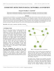
The communities at each time step were extracted with the Clique Percolation Method (CPM) [23, 24], defining a community as a union of all k-cliques (complete subgraphs of size k) that can be reached from each other through a series of adjacent k-cliques (where adjacency means sharing k − 1 nodes) [24,28,29]. When applied to weighted networks, the CPM has two parameters: the k-clique size k, (in Fig.1a-b we show the communities for k = 4), and the weight threshold w∗ (links weaker than w∗ are ignored). By increasing k or w∗ , the communities start to shrink and fall apart, but at the same time they become also more cohesive. In the opposite case, at low k there is a critical w∗ , under which a giant community appears in the system that smears out the details of the community structure by merging (and making invisible) many smaller communities. The criterion used to fix these parameters is based on finding a community structure as highly structured as possible: at the highest k value for which a giant community may emerge, the w∗ is decreased just below the critical point. The actual values of these parameters in our studies were k = 3, w∗ = 0.1 in case of the co-authorship network, and k = 4, w∗ = 1.0 in case of the phone-call network. The key feature of the communities obtained by the CPM are that (i) their members can be reached through well connected subsets of nodes, and (ii) the communities may overlap (share nodes with each other). This latter property is essential, since most networks are characterized by overlapping and nested communities [5, 23]. In Fig.1a-b we show the local structure at a given time step in the two networks in the vicinity of a randomly chosen individual (marked by a red frame). The communities (social groups represented by more densely interconnected parts within a network of social links) are color coded, so that black nodes/edges do not belong to any community, and those that simultaneously belong to two or more communities are shown in red. The two networks have rather different local structure: due to its bipartite nature, the collaboration network is quite dense and the overlap between communities is very significant, whereas in the phone-call network the communities are less interconnected and are often separated by one or more inter-community nodes/edges. Indeed, while the phone record captures the communication between two people, the publication record assigns to all individuals that contribute to a paper a fully connected clique. As a result, the phone data is dominated by single links, while the co-authorship data has many dense, highly con-

Community dynamics in social networks

nected neighborhoods. Furthermore, the links in the phone network correspond to instant communication events, capturing a relationship as is happens. In contrast, the co-authorship data records the results of a long term collaboration process. These fundamental differences suggest that any potential common features of the community evolution in the two networks potentially, represent generic characteristics of community formation, rather than being rooted in the details of the network representation or data collection process. As a first step, it is important to check if the uncovered communities correspond to groups of individuals with a shared common activity pattern. For this purpose we compared the average weight of the links inside communities, wc , to the average weight of the inter-community links, wic . For the co-authorship network wc /wic is about 2.9, while for the phone-call network the difference is even more significant, since wc /wic ≃ 5.9, indicating that the intensity of collaboration/communication within a group is significantly higher than with contacts belonging to a different group [30–33]. While for coauthors the quality of the clustering can be directly tested by studying their publication records in more detail, in the phone-call network personal information is not available. In this case the zip-code and the age of the users provides additional information for checking the homogeneity of the communities. In Fig.1c we show the size of the largest subset of people having the same zip code in the communities, hnreal i, averaged over the time steps, as the function of the community size s, divided by hnrand i, representing the average over random sets of users. The significantly higher number of people with the same zip-code in the CPM communities as compared to random sets indicates that the communities usually correspond to individuals living relatively close to each other. It is of specific interest that hnreal i / hnrand i has a prominent peak at s ≃ 35, suggesting that communities of this size are geographically the most homogeneous ones. However, as Fig.1d shows, the situation is more complex: on average, the smaller communities are more homogeneous, but there is still a noticeable peak at s ≃ 30 − 35. In Fig.1c we also show the average size of the largest subset of members with an age falling into a three years wide time window, divided by the same quantity obtained for randomly selected groups of individuals. The fact that the ratio is larger than one indicates that communities have a tendency to contain people from the same generation, and the hnrand i /s plot indicates that the homogeneity of small groups is on average larger than that of the big groups. In summary, the phone-call communities uncovered by the CPM tend to contain individuals living in the same neighborhood, and with comparable age, a homogeneity that supports the validity of the uncovered community structure. (Further support is given in the Supplementary Material of Ref. 25). 3.2.

Evolving communities

The basic events that may occur in the life of a community are shown in Fig.1e: a community can grow by recruiting new members, or contract by loosing members; two (or more) groups may merge into a single community, while a large enough social group can split into several smaller ones; new communities are born and old ones may disappear. Given that community finding algorithms extract only static “snap-

Palla, Barab´ asi and Vicsek

a)

b)

co−authorship

phone−call

d) 0.6

c) 14

< nreal > < nrand >

0.5

zip−code age

12 10

0.4

8

< nreal > 0.3 s

6

zip−code age

0.2 4 0.1

2 0

0

e)

20

40

60

80

s

growth

t

100

contraction

t+1 merging

t

0

120

t+1

t

40

60

s

80

100

120

t+1 splitting

t

birth

20

f)

t t

0

t U t+1

t+1

t+1 death

t+1

t

t+1

Fig 1. a) The local community structure at a given time step in the vicinity of a randomly selected node in case of the co-authorship network. b) The same picture in the phone-call network. c) The black symbols correspond to the average size of the largest subset of members with the same zip-code, hnreal i, in the phone-call communities divided by the same quantity found in random sets, hnrand i, as the function of the community size s. Similarly, the white symbols show the average size of the largest subset of community members with an age falling in a three year time window, divided by the same quantity in random sets. The error-bars in both cases correspond to hnreal i /(hnrand i + σrand ) and hnreal i /(hnrand i − σrand ), where σrand is the standard deviation in case of the random sets d) The hnreal i /s as a function of s, for both the zip-code (black symbols) and the age (white symbols). e) Possible events in the community evolution. f) The identification of evolving communities. The links at t (blue) and the links at t + 1 (yellow) are merged into a joint graph (green). Any CPM community at t or t + 1 is part of a CPM community in the joined graph, therefore, these can be used to match the two sets of communities.

shots” of the community structure, and that a huge number of groups are present at each time step, it is a significant algorithmic and computational challenge to match communities uncovered at different time steps. The basic idea of the algorithm developed by us to identify community evolution is shown in Fig.1f. For each

Community dynamics in social networks

consecutive time steps t and t + 1 we construct a joint graph consisting of the union of links from the corresponding two networks, and extract the CPM community structure of this joint network (we thank I. Der´enyi for pointing out this possibility). Any community from either the t or the t + 1 snap-shot is contained in exactly one community in the joint graph, since by adding links to a network, the CPM communities can only grow, merge or remain unchanged. Thus, the communities in the joint graph provide a natural connection between the communities at t and at t + 1. If a community in the joint graph contains a single community from t and a single community from t + 1, then they are matched. If the joint group contains more than one community from either time steps, the communities are matched in descending order of their relative node overlap, which is defined for a pair of communities A and B as |A ∩ B| , (2) C(A, B) ≡ |A ∪ B| where |A ∩ B| is the number of common nodes in A and B, and |A ∪ B| is the number of nodes in the union of the two communities. (For more details, see the Supplementary Information of Ref. 25). 4. 4.1.

Statistical properties of the community dynamics Basic statistics

One of the most basic properties characterizing the partitioning of a network is the overall coverage of the community structure, i.e. the ratio of nodes contained in at least one community. In case of the co-authorship network the average value of this ratio was above 59%, which is a reasonable coverage for the CPM. In contrast, we could only achieve a significantly smaller ratio for the phone-call network. At such a large system size, in order to be able to match the communities at subsequent time steps in reasonable time we had to decrease the number of communities by choosing a higher k and w∗ parameter (k = 4 and w∗ = 1.0), and keeping only the communities having a size larger or equal to s = 6. Therefore, in the end the ratio of nodes contained in at least one community was reduced to 11%. However, this still means more than 400000 customers in the communities on average, providing a representative sampling of the system. By lowering the k to k = 3, the fraction of nodes included in the communities is raised to 43%. Furthermore, a significant number of additional nodes can be also classified into the discovered communities. For example, if a node not yet classified has link(s) only to a single community (and, if it has no links connecting to nodes in any other community) it can be safely added to that community. Carrying out this process iteratively, the fraction of nodes that can be classified into communities increases to 72% for the k=3 coauthorship network, and to 72% (61%) for the k=3 (k=4) mobile phone network, which, in principle, allows us to classify over 2.4 million users into communities. Another important statistics describing the community system is the community size distribution. In Fig.2a we show the community size distribution in the phonecall network at different time steps. They all resemble to a power-law with a high exponent. In case of t = 0, the largest communities are somewhat smaller than in the later time steps. This is due to the fact that the events before the actual time step cannot contribute to the link-weights in case of t = 0, whereas they can if t > 0.

Palla, Barab´ asi and Vicsek a)

b)

phone−call

co−authorship

1

1 t=0 t=5 t=10 t=15

10 −1

t=0 t=15 t=30 t=60 t=90 t=120

10 −1

10 −2 P(s)

−2 P(s)10

10 −3

10 −3

10 −4 10 −5

1

c)

10

10 10

3

N(s) 10

2

1

d)

phone−call 4

10 −4

10 2

s

10

s

co−authorship t=0 t=15 t=30 t=60 t=90 t=120

10 3 t=0 t=5 t=10 t=15

10 2

10 2 N(s) 10

10

1

1 1

10

s

10 2

1

10

s

10 2

Fig 2. a) The cumulative community size distribution in the phone-call network at different time steps. b) The time evolution of the cumulative community size distribution in the co-authorship network. c) The number of communities of a given size at different time steps in the phone-call network. d) The time evolution of the number of communities with a given size in the co-authorship network.

In Fig.2b we can follow the time evolution of the community size distribution in the co-authorship network. In this case t = 0 corresponds to the birth of the system itself as well (whereas in case of the phone-calls it does not), therefore the network and the communities in the network are small in the first few time steps. Later on, the system is enlarged, and the community size distribution is stabilized close to a power-law. In Figs.2c-d we show the number of communities as a function of the community size at different time steps in the examined systems. For the phone-call network (Fig.2c), this distribution is more ore less constant in time. In contrast, (due to the growth of the underlying network) we can see an overall growth in the number of communities with time in the co-authorship network (Fig.2d). Since the number of communities drops down to only a few at large community sizes in both systems, we used size binning when calculating the statistics shown in Sect.4.2 and Sect.4.4. 4.2.

Correlations, stationarity and expected life-time

As for evolving communities, we first consider two basic quantities characterizing a community: its size s and its age τ , representing the time passed since its birth. s and τ are positively correlated: larger communities are on average older (Fig.3a), which is quite natural, as communities are usually born small, and it takes time

Community dynamics in social networks

to recruit new members to reach a large size. Next we used the auto-correlation a)

3 2.8 2.6 2.4 2.2 < τ(s ) > 2 < τ > 1.8 1.6 1.4 1.2 1 0.8

b)

c)

60 50

25

s

40 20

30

15

20 10

10

0

20

40

60

s

80

100

120

d)

phone−call, phone−call, phone−call, co−authorship, co−authorship, co−authorship,

0.8 0.7 0.6

5 0.8

140

1 s=6 s=12 s=18 s=6 s=12 s=18

0.4 0.3 0.2 5

10

15

20

t

25

30

0.825 0.85 0.875

0.9

ζ

0.925 0.95 0.975

1

18

< τ *> 20

14

s

0

0

16

0.5

0.1

< τ *>

30

0.9

< C(t )>

35

co−authorship phone−call

35

40

15

12

10

10

5

8

0

6 0.85

0.875

0.9

0.925

ζ

0.95

0.975

1

Fig 3. a) The average age τ of communities with a given size (number of people) s, divided by the average age of all communities hτ i, as the function of s, indicating that larger communities are on average older. b) The average auto-correlation function C(t) of communities with different sizes (the unit of time, t, is one month). The C(t) of larger communities decays faster. c) The average life-span hτ ∗ i of the communities as the function of the stationarity ζ and the community size s for the co-authorship network. The peak in hτ ∗ i is close to ζ = 1 for small sizes, whereas it is shifted towards lower ζ values for large sizes. d)Similar results found in the phone-call network.

function, C(t), to quantify the relative overlap between two states of the same community A(t) at t time steps apart: CA (t) ≡

|A(t0 ) ∩ A(t0 + t)| , |A(t0 ) ∪ A(t0 + t)|

(3)

where |A(t0 ) ∩ A(t0 + t)| is the number of common nodes (members) in A(t0 ) and A(t0 + t), and |A(t0 ) ∪ A(t0 + t)| is the number of nodes in the union of A(t0 ) and A(t0 +t). Fig.3b shows the average time dependent auto-correlation function for communities born with different sizes. We find that in both networks, the auto-correlation function decays faster for the larger communities, indicating that the membership of the larger communities is changing at a higher rate. On the contrary, small communities change at a smaller rate, their composition being more or less static. To quantify this aspect of community evolution, we define the stationarity ζ of a community as the average correlation between subsequent states: Ptmax −1 C(t, t + 1) ζ ≡ t=t0 , (4) tmax − t0 − 1 where t0 denotes the birth of the community, and tmax is the last step before the extinction of the community. In other words, 1 − ζ represents the average ratio

Palla, Barab´ asi and Vicsek

of members changed in one step; larger ζ corresponds to smaller change (more stationary membership). We observe a very interesting effect when we investigate the relationship between the lifetime τ ∗ (the number of steps between the birth and disintegration of a community), the stationarity and the community size. The lifetime can be viewed as a simple measure of “fitness”: communities having higher fitness have an extended life, while the ones with small fitness quickly disintegrate, or are swallowed by another community. In Fig.3c-d we show the average life-span hτ ∗ i (color coded) as a function of the stationarity ζ and the community size s (both s and ζ were binned). In both networks, for small community sizes the highest average life-span is at a stationarity value very close to one, indicating that for small communities it is optimal to have static, time independent membership. On the other hand, the peak in hτ ∗ i is shifted towards low ζ values for large communities, suggesting that for these the optimal regime is to be dynamic, i.e., a continually changing membership. In fact, large communities with a ζ value equal to the optimal ζ for small communities have a very short life, and similarly, small communities with a low ζ (being optimal at large sizes) are disappearing quickly as well. a)

τ=0−2

50

s

τ=3

τ=4−34

τ=35

τ=36−52

small, stationary 0

0

10

20

30

τ

40

50

b) 50 τ=1

s 0

c)

τ=2

τ=3

τ=4

τ=5

τ=6

τ=7

τ=8

small, non−stationary 0

10

20

τ

30

40

50

20

τ

30

40

50

50 large, stationary

s 0

0

d)

10 new

200

old

e)

leaving in next step

large, non−stationary

150

s

100 50 0

0

10

20

τ

30

40

50

τ=9

τ=10

Fig 4. Time evolution of four communities in the co-authorship network. The height of the columns corresponds to the actual community size, and within one column the yellow color indicates the number of ”old” nodes (that have been present in the community at least in the previous time step as well), while newcomers are shown with green. The members abandoning the community in the next time step are shown with orange or purple color, depending on whether they are old or new. (This latter type of member joins the community for only one time step). From top to bottom, we show a small and stationary community (a), a small and non-stationary community (b), a large and stationary community (c) and, finally, a large and non-stationary community (d). A mainly growing stage (two time steps) in the evolution of the latter community is detailed in panel e).

To illustrate the difference in the optimal behavior (a pattern of membership dynamics leading to extended lifetime) of small and large communities, in Fig.4. we show the time evolution of four communities from the co-authorship network.

Community dynamics in social networks

As Fig.4. indicates, a typical small and stationary community undergoes minor changes, but lives for a long time. This is well illustrated by the snapshots of the community structure, showing that the community’s stability is conferred by a core of three individuals representing a collaborative group spanning over 52 months. While new co-authors are added occasionally to the group, they come and go. In contrast, a small community with high turnover of its members, (several members abandon the community at the second time step, followed by three new members joining in at time step three) has a lifetime of nine time steps only (Fig.4b). The opposite is seen for large communities: a large stationary community disintegrates after four time steps (Fig.4c). In contrast, a large non-stationary community whose members change dynamically, resulting in significant fluctuations in both size and the composition, has quite extended lifetime (Fig.4d). Indeed, while the community undergoes dramatic changes, gaining (Fig.4e) or loosing a high fraction of its membership, it can easily withstand these changes.

4.3.

Commitment and life-time

The quite different stability rules followed by the small and large communities raise an important question: could an inspection of the community itself predict its future? To address this question, for each member in a community we measured the total weight of this member’s connections to outside of the community (wout ) as well as to members belonging to the same community (win ). We then calculated the probability that the member will abandon the community as a function of the wout /(win + wout ) ratio. As Fig.5a shows, for both networks this probability increases monotonically, suggesting that if the relative commitment of a user is to individuals outside a given community is higher, then it is more likely that he/she will leave the community. In parallel, the average time spent in the community by the nodes, hτn i, is a decreasing function of the above ratio (Fig.5a inset). Individuals that are the most likely to stay are those that commit most of their time to community members, an effect that is particularly prominent for the phone network. As Fig.5a shows, those with the least commitment have a quickly growing likelihood of leaving the community. Taking this idea from individuals to communities, we measured for each community the total weight of links (a measure of how much a member is committed) from the members to others, outside of the community (Wout ) , as well as the aggregated link weight inside the community (Win ). We find that the probability for a community to disintegrate in the next step increases as a function of Wout /(Win + Wout ) (Fig.5b), and the lifetime of a community decreases with the Wout /(Win + Wout ) ratio (Fig.5b inset). This indicates that self-focused communities have a significantly longer lifetime than those that are open to the outside world. However, an interesting observation is that, while the lifetime of the phone-call communities for moderate levels is relatively insensitive to outside commitments, the lifetime of the collaboration communities possesses a maximum at intermediate levels of inter-collaborations (collaboration between colleagues who belong to different communities). These results suggest that a tracking of the individual’s as well as the community’s relative commitment to the other members of the community provides a clue for predicting the community’s fate.

Palla, Barab´ asi and Vicsek

a) 0.08

b) 16

0.2

35 30

14

0.07

12

0.06

τn

0.05

pl

τ∗

8 6

pd

4

0.04

2 0

0.03 0.02

wout/(win+ wout ) 0

0.1 0.2 0.3 0.4 0.5 0.6 0.7 0.8 0.9

0

0.1

0.2

0.3

20 15 10

0.1

5

Wout /(Win + Wout )

0 0 0.1 0.2 0.3 0.4 0.5 0.6 0.7 0.8 0.9 1

1

0.05

co−authorship phone−call

0.01 0

25

0.15

10

co−authorship phone−call 0.4

0.5

0.6

wout / (win + wout)

0.7

0.8

0.9

1

0

0

0.1

0.2

0.3

0.4

0.5

0.6

Wout /(Win +Wout )

0.7

0.8

0.9

1

Fig 5. a) The probability pℓ for a member to abandon its community in the next step as a function of the ratio of its aggregated link weights to other parts of the network (wout ) and its total aggregated link weight (win +wout ). The inset shows the average time spent in the community by the nodes, hτn i, in function of wout /(win + wout ). b) The probability pd for a community to disintegrate in the next step in function of the ratio of the aggregated weights of links from the community to other parts of the network (Wout ) and the aggregated weights of all links starting from the community (Win + Wout ). The inset shows the average life time hτ ∗ i of communities as a function of Wout /(Win + Wout ).

4.4.

Merging of communities

During the time evolution, a pair (or a larger group) of initially distinct communities can join together to form a single community. A very interesting question connected to this is that can we find a simple relation between the size of a community and the likelihood that it will take part in such process? To investigate this issue we carried out measurements similar to those in Ref. [21]. The basic idea is that if the merging process is uniform with respect to the size of the communities s, then communities with a given s are chosen at a rate given by the size distribution of the available communities. However, if the merging mechanism prefers large (or small) sizes, then communities with large (or small) s are chosen with a higher rate compared to the size distribution of the available communities. To monitor this enhancement, at each time step t the cumulative size-pair distribution Pt (s1 , s2 ) was recorded. Simultaneously, the un-normalized cumulative size-pair distribution of the communities merging between t and t+1 was constructed; we shall denote this distribution by wt→t+1 (s1 , s2 ). The value of this rate-like variable wt→t+1 (s∗1 , s∗2 ) at a given value of s∗1 and s∗2 is equal to the number of pairs of communities that merged between t and t + 1 and had sizes s1 > s∗1 and s2 > s∗2 . To detect deviations from uniform merging probabilities, the ratio of wt→t+1 (s1 , s2 ) and Pt (s1 , s2 ) was accumulated during the time evolution resulting in W (s1 , s2 ) ≡

tmax X−1 t=0

wt→t+1 (s1 , s2 ) . Pt (s1 , s2 )

(5)

When the merging process is uniform with respect to the community size the W (s1 , s2 ) becomes a flat function: on average we see pairs of communities merging with sizes s1 and s2 at a rate equal to the probability of finding a pair of communities of these sizes. However, if the merging process prefers large (or small) communities, than pairs with large (or small) sizes merge at a higher rate than the

Community dynamics in social networks

probability of finding such pairs, and W (s1 , s2 ) becomes increasing (or decreasing) with the size. The reason for using un-normalized wt→t+1 (s1 , s2 ) distributions is that in this way each merging event contributes to W (s1 , s2 ) with equal weight, and the time steps with a lot of merging events count more than those with only a few events. In the opposite case, (when wt→t+1 (s1 , s2 ) is normalized for each pairs of subsequent time steps t, t + 1), the merging events occurring between time steps with a lot of other merging events are suppressed compared to the events with only a few other parallel events, as each pairs of consecutive time steps t, t + 1 contribute to the W (s1 , s2 ) function with equal weights. This difference between normalized and unnormalized wt→t+1 (s1 , s2 ) becomes important in case of the co-authorship network, where in the beginning the system is small and merging is rare, and later on as the system is developing, merging between communities becomes a regular event. In Fig.6. we show W (s1 , s2 ) for both networks, and the picture suggests that large sizes are preferred in the merging process. This is consistent with our findings a)

b)

co−authorship

phone−call

60 50 40

s 2 30 20 10

W(s1,s2)

30

6e+05 5e+05 4e+05 3e+05 2e+05 1e+05 0

25

15 10 10

s1 d) W(s1,s2)

25

4e+05

20

3e+05

s 2 15

2e+05 1e+05

10

0 5 5

10 15 20 25 30

s1

15

20

25

30

s1

co−authorship 30

5e+06 4e+06 3e+06 2e+06 1e+06 0

s 2 20

10 20 30 40 50 60

c)

W(s1,s2)

phone−call W(s1,s2)

20 18 16 14 s2 12 10 8 6

3e+06 2e+06 1e+06 0 6 8 10 12 14 16 18 20

s1

Fig 6. The merging of communities. a) the W (s1 , s2 ) function for the co-authorship network, b) the W (s1 , s2 ) function for the phone-call network, c) the region with smaller W (s1 , s2 ) in (a) enlarged, d) the region with smaller W (s1 , s2 ) in (b) enlarged.

that the content of large communities is changing at a faster rate compared to the small ones. Swallowing other communities is an efficient way to bring numerous new members into the community in just one step, therefore taking part in merging is beneficial for large communities following a survival strategy based on constantly changing their members. Another interesting aspect of the results shown in Fig.6. is that they are analogous to the attachment mechanism of links between already existing nodes in collaboration networks [11]: the probability for a new link to

Palla, Barab´ asi and Vicsek

appear between two nodes with degree d1 and d2 is roughly proportional to d1 × s2 . Similarly, the probability that two communities of sizes s1 and s2 will merge is proportional to to s1 × s2 , therefore the large communities attract each other in a similar manner to hubs in collaboration networks. 5.

Summary and conclusion

In summary, our results indicate a significant difference between smaller collaborative or friendship circles and institutions. At the heart of small cliques are a few strong relationships, and as long as these persist, the community around them is stable. It appears to be almost impossible to maintain this strategy for large communities, however. Thus we find that the condition for stability for large communities is continuous changes in their membership, allowing for the possibility that after some time practically all members are exchanged. Such loose, rapidly changing communities are reminiscent of institutions, that can continue to exist even after all members have been replaced by new members. For example, in a few years most members of a school or a company could change, yet the school and the company will be detectable as a distinct community at any time step during its existence. We also showed that the knowledge of the time commitment of the members to a given community can be used for predicting the community’s lifetime. Furthermore, we found that the likelihood of merging between communities is increasing with the community size. These findings offer a new view on the fundamental differences between the dynamics of small groups and large institutions. Acknowledgements We thank I. Der´enyi for useful suggestions, G. Szab´o and I. Farkas for their assistance with the primary phone-call and co-authorship datasets, respectively. G.P and T.V are supported by grants from OTKA Nos: K068669 and T034995; A.L.B is supported by the James S. McDonnell Foundation and the National Science Foundation ITR DMR-0426737 and CNS-0540348 within the DDDAS program. References [1] D. J. Watts and S. H. Strogatz. Collective dynamics of ’small-world’ networks. Nature, 393:440–442, 1998. [2] A.-L. Barab´ asi and R. Albert. Emergence of scaling in random networks. Science, 286:509–512, 1999. [3] J. Scott. Social Network Analysis: A Handbook, 2nd ed. Sage Publications, London, 2000. [4] D. J. Watts, P. S. Dodds, and M. E. J. Newman. Identity and search in social networks. Science, 296:1302–1305, 2002. [5] K. Faust. Using correspondence analysis for joint displays of affiliation networks. In P.Carrington, J. Scott, and S. Wasserman, editors, Models and Methods in Social Network Analysis, chapter 7. Cambridge University Press, New York, 2005. [6] F. Liljeros, Ch. R. Edling, L. A. N. Amaral, H. E. Stanley, and Y. Aberg. The web of human sexual contacts. Nature, 411:907–908, 2001. [7] R. M. Shiffrin and K. B¨ orner. Mapping knowledge domains. Proc. Natl. Acad. Sci. USA, 101:5183–5185 Suppl. 1, 2004.

Community dynamics in social networks

[8] M. E. J. Newman. Detecting community structure in networks. Eur. Phys. J. B, 38:321–330, 2004. [9] M. Girvan and M. E. J. Newman. Community structure in social and biological networks. Proc. Natl. Acad. Sci. USA, 99:7821–7826, 2002. [10] F. Radicchi, C. Castellano, F. Cecconi, V. Loreto, and D. Parisi. Defining and identifying communities in networks. Proc. Natl. Acad. Sci. USA, 101:2658–2663, 2004. [11] A.-L. Barab´ asi, H. Jeong, Z. N´eda, E. Ravasz, A. Schubert, and T. Vicsek. Evolution of the social network of scientific collaborations. PHYSICA A, 311:590–614, 2002. [12] P. Holme, Ch. R. Edling, and F. Liljeros. Structure and time-evolution of an internet dating community. Social Networks, 26:155–174, 2004. [13] H. Ebel, J. Davidsen, and S. Bornholdt. Dynamics of social networks. Complexity, 8:24–27, 2002. [14] C. S. Wagner and L. Leydesdorff. Network structure, self-organization, and the growth of international collaboration in science. Research Policy, 34:1608–1618, 2005. [15] Y.-Y. Yeung, T. C.-Y. Liu, and P.-H. Ng. A social network analysis of research collaboration in physics education. American Journal of Physics, 73:145–150, 2005. [16] M. E. J. Newman and J. Park. Why social networks are different from other types of networks. Phys. Rev. E, 68:036122, 2003. [17] R. Guimer´ a, L. Danon, A. Diaz-Guilera, F. Giralt, and A. Arenas. Self-similar community structure in organisations. Physical Review E, 68:065103, 2003. [18] J. Hopcroft, O. Khan, B. Kulis, and B. Selman. Tracking evolving communities in large linked networks. Proc. Natl. Acad. Sci. USA, 101:5249–5253, 2004. [19] R. Guimer´ a, B. Uzzi, J. Spiro, and L. A. N. Amaral. Team assembly mechanisms determine collaboration network structure and team performance. Science, 308:697– 702, 2005. [20] Ch. Li and Ph. K. Maini. An evolving network model with community structure. Journal of Physics A: Mathematical and General, 38:9741–9749, 2005. [21] P. Pollner, G. Palla, and T. Vicsek. Preferential attachment of communities: The same principle, but a higher level. Europhys. Lett., 73:478–484, 2006. [22] G. Kossinets and D. J. Watts. Empirical analysis of an evolving social network. Science, 311:88–90, 2006. [23] G. Palla amd I. Der´enyi, I. Farkas, and T. Vicsek. Uncovering the overlapping community structure of complex networks in nature and society. Nature, 435:814–818, 2005. [24] I. Der´enyi, G. Palla, and T. Vicsek. Clique percolation in random networks. Phys. Rev. Lett., 94:160202, 2005. [25] G. Palla, A.-L. Barab´ asi, and T. Vicsek. Quantifying social group evolution. Nature, 446:664–667, 2007. [26] S. Warner. E-prints and the open archives initiative. Library Hi Tech, 21:151–158, 2003. [27] J. J. Ramasco and S. A. Morris. Social inertia in collaboration networks. Phys. Rev. E, 73:016122, 2006. [28] M. G. Everett and S. P. Borgatti. Analyzing clique overlap. Connections, 21:49–61, 1998. [29] V. Batagelj and M. Zaversnik. Short cycles connectivity. Preprint at http://arxiv.ogr/abs/cs.DS/0308011, 2003. [30] M. S. Granovetter. The strength of weak ties. American Journal of Sociology, 78:1360– 1380, 1973.

Palla, Barab´ asi and Vicsek

[31] P. Csermely. Weak Links. Springer Verlag, Heidelberg, Germany, 2006. [32] J.-P. Onnela, J. Saramaki, J. Hyvonen, G. Szab´ o, D. Lazer, K. Kaski, J. Kert´esz, and A.-L. Barabasi. Structure and tie strengths in mobile communication networks. To appear in Proc. Nat. Acad. Sci. (PNAS Article 06-10245), preprint at http://arxiv.org/abs/physics/0610104v1, 2006. [33] J.-P. Onnela, J. Saramaki, J. Hyvonen, G. Szab´ o, M. Argollo de Menezes, K. Kaski, A.-L. Barab´ asi, and J. Kertesz. Analysis of a large-scale weighted network of oneto-one human communication. to appear in New Journal of Physics, preprint at http://arxiv.org/abs/physics/0702158, 2007.