Commodity Price Responses to Monetary Policy Surprises Dean Scrimgeour∗ Colgate University 14 April, 2010

Abstract Commodity prices are important both as a source of shocks and for the propagation of shocks originating elsewhere in the economy. Many vector autoregression (VAR) studies estimate a gradual response of commodity prices to monetary policy shocks. Exploiting information in high-frequency financial market data, and using the methods of Rigobon and Sack (2004) I find that a 10 basis point surprise change in interest rates causes commodity prices to fall immediately by about 0.5%. This is about two-thirds of the estimated response of the S&P500, and about five times larger than the response in a VAR 12 months after the shock. Metals prices tend to respond more than agricultural commodities. The point estimate for oil prices is similar to other commodities, but is estimated imprecisely.

∗

Contact: Dean Scrimgeour, Economics Department, Colgate University, 13 Oak Drive, Hamilton, NY 13346. Email: [email protected]. This work has benefited from comments from Emily Conover, Ed Gamber, Chad Jones, Yuriy Gorodnichenko, Roisin O’Sullivan, Ann Owen, Christina Romer, David Romer, Nicole Simpson, Julie Smith, Chad Sparber, and Marc Tomljanovich. Thanks also to RC Research for providing futures data.

2

1.

DEAN SCRIMGEOUR

Introduction

I explore the influence of monetary policy on commodity prices. Since commodity prices help determine a wide range of consumer and producer prices, the response of commodity prices to monetary policy may be an important aspect of the monetary transmission mechanism. The relationship between commodity prices and monetary policy has been given a lot of attention over the years. Some blame the inflation of the 1970s on rising commodity prices (see for example, Blinder, 1982). By contrast Barsky and Kilian (2001) argue that commodity prices tended to rise in the 1970s in response to anticipated inflation brought on by loose monetary policy. During the 2005-2008 period, elevated commodity prices brought renewed attention to commodity markets. Would high oil prices lead to inflation? Would they cause a recession? Would they generate both, returning the economy to stagflation as in the 1970s? Explanations for why commodity prices have been high include growing demand in China and speculative behavior in financial markets (Hamilton, 2009). In addition, revisiting Barsky and Kilian (2001), Taylor (2009) has argued that loose monetary policy may be behind the surge in commodity prices. This paper attempts to measure the size of monetary policy surprises’ effects on commodity prices. Like other financial market prices, commodity prices are relatively flexible, adjusting quickly in response to shocks. Any effects of monetary policy announcements on commodity prices likely occur within a short period of the announcement, by contrast with retail prices, which are stickier. I study the relationship between commodity prices and interest rates around particular news-related events. The event days are when the Federal Reserve’s Open Markets Committee meets and financial markets acquire new information about the course of monetary policy. The paper is related to Cook and Hahn (1989) who focused on meeting dates to measure the response of bond markets to changes in the Federal Reserve’s target federal funds rate. However, Cook and Hahn’s study ignores the fact that financial market participants learn about more than just monetary policy on these event days. Rigobon and Sack (2004), whose method I implement, account for the fact that other forces may move both interest rates and asset prices on event days, confounding the event study estimator. They show how to estimate the effect of monetary policy on asset prices

COMMODITY PRICES AND MONETARY POLICY

3

using instrumental variables techniques that rely on non-event days to provide information about the typical relationship between interest rates and commodity prices. Deviation from this normal relationship on event days is interpreted as being due to monetary policy surprises. The results in this paper indicate a rapid, statistically significant, and economically significant response of commodity prices to monetary policy. Point estimates suggest that a 10 basis point increase in interest rates would cause commodity prices to fall by approximately 0.5% immediately. This finding poses a challenge for vector autoregression (VAR) studies that impose the restriction that commodity prices can only respond to monetary policy surprises from previous months or quarters (Christiano et al., 1999). In a standard recursively-identified VAR, a 10 basis point surprise increase in interest rates would lower commodity prices by approximately 0.1% after a year, with smaller responses closer to the timing of the surprise. Section 2 discusses related literature. Section 3 reviews the empirical approach. Section 4 presents results, and section 5 concludes.

2.

Related Work

Monetary policy affects asset prices, including commodity prices, in a variety of ways. Commodities and bonds are substitutes as assets that store value. When the Federal Reserve sells bonds to raise interest rates, demand for commodities falls. Therefore commodity prices should fall when interest rates rise due to monetary intervention. Other shocks, such as new information about bond risk, might move bond prices and commodity prices in opposite directions. Taylor (2009) presents a monetary explanation for the recent peaks in commodity prices. He argues that oil prices increased in 2007 and 2008 because the Federal Open Market Committee (FOMC) reduced in interest rates. Similarly Frankel (2008) has argued that reductions in interest rates could increase commodity prices. In his work he emphasizes an overshooting mechanism in the response of commodity prices to monetary policy.1 The overshooting story aims to explain the magnitude of the rise in 1

See also Frankel (1984); Frankel and Hardouvelis (1985); Frankel (1986).

4

DEAN SCRIMGEOUR

commodity prices in response to a monetary policy surprise.2 Consistent with weak forms of the efficient markets hypothesis, I assume the effect of monetary policy surprises occurs on the day the surprises occur. In the Dornbusch (1976) model, the large movement of the asset price happens exactly at the moment of the shock. There are no predictable jumps in the asset price after this point. An arbitrage relationship equates the expected returns on bonds and other safe assets (c.f. Hotelling, 1931). To see the influence of monetary policy on commodity prices, consider the following stripped-down, continuous-time version of the Dornbusch-Frankel model. Monetary policy is described by an interest rate rule 𝑖𝑡 = ¯𝑖 + 𝜓(𝑝𝑡 − 𝑝¯),

𝜓>0

where 𝑝𝑡 is the level of consumer prices, for which the central bank has a target of 𝑝¯. When the price level is above its target, the central bank sets interest rates above the long-run average interest rate ¯𝑖. Consumer prices adjust gradually toward the target level 𝑝˙𝑡 = −𝜃(𝑝𝑡 − 𝑝¯),

𝜃>0

since when the price level is above the target, monetary policy is tight and inflation is low. When the price level is below the target, monetary policy is loose, and inflation is high. Intertemporal optimization in the supply of commodities implies the Hotelling rule, that 𝑝˙𝑐𝑜𝑚,𝑡 = 𝑖𝑡 where 𝑝𝑐𝑜𝑚 is the commodity price. Consumer prices are predetermined, but commodity prices are flexible. In the long run, commodity prices and consumer prices are equal 𝑝𝑡 = 𝑝𝑐𝑜𝑚,𝑡 .

2 Caballero et al. (2008a,b) also link interest rates and commodity prices, noting that commodity prices have been high at the same time real interest rates have been low in recent years. They emphasize a global savings glut (Bernanke, 2005) to explain levels of interest rates and commodity prices. During the early stages of the financial crisis, when debt began looking riskier, there was a sell-off in bonds and investors substituted some commodities for bonds in their portfolios.

COMMODITY PRICES AND MONETARY POLICY

5

Assuming that ¯𝑖 = 0 the model’s solution is straightforward: 𝑝𝑡 = (𝑝0 − 𝑝¯)𝑒−𝜃𝑡 + 𝑝¯

𝑝𝑐𝑜𝑚,𝑡

= 𝑝¯(1 − 𝑒−𝜃𝑡 ) + 𝑝0 𝑒−𝜃𝑡 𝜓 = 𝑝¯ − (𝑝0 − 𝑝¯)𝑒−𝜃𝑡 𝜃 𝜓 𝜓 = 𝑝¯(1 + )𝑒−𝜃𝑡 − 𝑝0 𝑒−𝜃𝑡 𝜃 𝜃

(1) (2) (3) (4)

where 𝑝0 is the initial, predetermined consumer price level. An unexpected increase in 𝑝¯ causes a fall in interest rates. The consumer price level 𝑝 does not move when the shock occurs but the commodity price does. The lower interest rate causes the commodity price to rise. The commodity price overshoots, rising more in the short run than the long run. (The short run effect on 𝑝𝑐𝑜𝑚 of a one unit change in 𝑝¯ is (1 + 𝜓𝜃 ) > 1 while the long run effect is 1.) Consider an unexpected, permanent change in the consumer price level target at time zero. The effect on the commodity price level is largest when the shock occurs ∂𝑝𝑐𝑜𝑚,𝑡 ∂ 𝑝¯ 2 ∂ 𝑝𝑐𝑜𝑚,𝑡 ∂𝑡∂ 𝑝¯

= 1+

𝜓 −𝜃𝑡 𝑒 >0 𝜃

= −𝜓𝑒−𝜃𝑡 < 0

so that there are implications for the term structure of commodity prices. Spot prices should move more than futures prices, and the difference between the responses is due to 𝜓 and 𝜃. This is the analog of Dornbusch’s overshooting result, and I test for it using an index of commodity price futures at various horizons. An alternative representation of the solution to the model gives the commodity price as a function of the entire path of future interest rates: ∫ 𝑝𝑐𝑜𝑚,𝑡 = 𝑝¯ −

∞

𝑖𝜏 𝑑𝜏. 0

According to this formulation short-lived deviations of interest rates from their equilibrium level will induce small movements in commodity prices. When the interest rate is away from its equilibrium level for a longer period, the effect on commodity prices

6

DEAN SCRIMGEOUR

is larger. Timing surprises are information about relatively short duration deviations of interest rates from their previously anticipated path, and so should have smaller effects on commodity prices. Timing surprises are unlikely to affect asset markets as much as surprises about the future level of interest rates. This is why it is important to measure monetary policy shocks in a way that separates timing surprises from level surprises. In measuring the effect of monetary policy surprises on commodity prices I follow Rigobon and Sack (2004) who modify the event study procedure to account for other (unknown) factors that may influence both interest rates and asset prices on event days. They apply these methods to estimate the effect of monetary policy surprises on stock and bond yields. Other studies using these methods have estimated the effects of monetary policy on stock prices, interest rates, and exchange rates.3 Mine is the only study to apply these methods to analyze the effect of monetary policy on commodity prices using high-frequency data.4 Following Rigobon and Sack, I measure monetary policy surprises using three-month Eurodollar futures. Since these are not spot rates, they are less affected by surprises due to the Fed adjusting its target rate a month earlier or later than expected (a timing surprise).5 I also use the Kuttner (2001) method as a robustness check. Kuttner’s work shows how to use federal funds futures contracts to measure monetary policy surprises.6 Conditional on accurate measurement of the surprise, assessing its effects on financial markets is relatively straightforward. The federal funds futures shock may capture important timing surprises related to when the Federal Reserve adjusts policy, so the federal funds futures shock mingles timing and level information. As in Kuttner, I use the spot 3

Craine and Martin (2008) apply the same approach to estimate the effect of U.S. policy surprises on Australian stocks and bonds and the USD/AUD exchange rate (as well as effects of Australian monetary policy surprises). 4 Frankel and Hardouvelis (1985) look at the commodity price response to weekly money supply announcements in the early 1980s, but give a different interpretation to the results. If commodity prices respond to the announcements, it is interpreted as evidence that the Federal Reserve’s previously announced monetary target is disregarded by market participants. If there is no response, this is interpreted to mean that markets regard the monetary surprise as an error in hitting the target rather than a change in the target. The methods in this paper, because they rely on forward-looking measures of policy, are not confounded by a targeting error. 5 Timing surprises relate to the level and slope of the yield curve. Significant monetary policy surprises affect the level of the yield curve (longer-term interest rates), whereas timing surprises affect the slope. For example, a change in the federal funds target rate that affects the anticipated rate in two weeks from the present but does not affect the anticipated rate three months into the future contains a timing surprise. The Kuttner method, since it uses primarily current month futures is more susceptible to timing surprises. 6 ¨ Gurkaynak et al. (2005) and Bernanke and Kuttner (2005), among others, follow this approach.

7

COMMODITY PRICES AND MONETARY POLICY

month federal funds futures contract to measure the shock, switching over to using the next month federal funds futures contract if an event day is within three days of the end of the month.

3.

Empirical Setup

Rigobon and Sack (2004) show how to modify the standard event study method to account for the endogeneity of the change in the interest rate. Consider estimating 𝛽 in Δ𝑝𝑡 = 𝛽Δ𝑖𝑡 + 𝜖𝑡

(5)

Δ𝑖𝑡 = 𝑚𝑝𝑡 + 𝜈𝑡

(6)

where Δ𝑝 is the change in the (log) price of an asset and Δ𝑖 is the change in an interest rate. Endogeneity problems arise because interest rates move for many reasons, even on event days, and these reasons may be related to other factors that affect asset prices (𝜖).7 In particular, 𝑚𝑝 is the monetary surprise, which is zero on non-event days but may be non-zero on events days. The shock 𝜈 may be correlated with 𝜖 causing Δ𝑖 to be endogenous in equation 5, even on event days. On event days the variance-covariance matrix of [Δ𝑝𝑡 , Δ𝑖𝑡 ]′ changes in a way that allows us to identify 𝛽. Rigobon and Sack show how to identify 𝛽 using an instrumental variables approach. The instrumental variable is defined as

𝑧𝑡 =

⎧   ⎨

Δ𝑖𝑡

  ⎩ −Δ𝑖𝑡

on event days on non-event days

and the equation is estimated using all the event days and the days immediately prior

7

As an application, the “policy surprise” measured from Federal Funds Futures contracts shows apparent surprises on non-event days as well as event days. It is likely that some of the movements in the Federal Funds Futures on non-event days (and possibly also on event days) represent the anticipated response of the Federal Reserve to news, rather than a monetary policy surprise.

8

DEAN SCRIMGEOUR

to the event days. Instrumental variables is consistent for 𝛽: 𝛽ˆ𝐼𝑉

=

𝑐𝑜𝑣(𝑧𝑡 , Δ𝑝𝑡 ) 𝑐𝑜𝑣(𝑧𝑡 , Δ𝑖𝑡 ) 1 1 2 2 2 2 (𝛽(𝜎𝑚𝑝 + 𝜎𝜈 ) + 𝜎𝜖,𝜈 ) − 2 (𝛽𝜎𝜈 + 𝜎𝜖,𝜈 )

=

𝛽

→

1 2 2 (𝜎𝑚𝑝

+ 𝜎𝜈2 ) − 12 𝜎𝜈2

2 𝑝 is the variance of the monetary policy surprise, 𝜎 2 is the variance of 𝜈, 𝜎 where 𝜎𝑚 𝜖,𝜈 is 𝜈

the covariance of 𝜖 with 𝜈, and we assume that monetary policy shocks 𝑚𝑝 are uncorrelated with either 𝜖 or 𝜈. Table 1 shows some summary statistics for changes in commodity prices and the three-month Eurodollar futures rate on event days (when the FOMC meets) and nonevent days.8 The variances of commodity price movements tend to be higher on event days, and the covariances with the interest rate tend to be more negative. I use all regularly scheduled Federal Open Market Committee meeting dates from 1994 to March 2008 as event days. This gives 114 event days. As a robustness check, I also look at FOMC chairs’ testimonies presented under the Humphrey-Hawkins regulation as additional event days as well as extending the sample of events back to 1989. I have daily data on seventeen commodities over this period. There are nine metals (gold, silver, copper, aluminum, tin, zinc, platinum, lead, and nickel)9 , seven agricultural commodities (cocoa, coffee, cotton, wheat, hogs, live cattle, and livestock), and oil. For each commodity I fail to reject the null hypothesis of a unit root in the log of the price level with a Phillips-Perron test. This is important, since it means the effects I estimate using daily data are likely to be long lasting, and will eventually affect output and consumer prices.

4.

Results

8

Variables in my data are recorded before the FOMC announcements come out, so the event day movements are for the difference between prices the day after the announcement and the day of the announcement. 9 Data for lead prices start in 1995.

COMMODITY PRICES AND MONETARY POLICY

4.1.

9

Response of Commodity Prices to Monetary Policy Surprises

Tables 2 and 3 show estimates of the effect of monetary policy surprises on commodity prices. Table 2 shows estimates when commodity prices are grouped together. The commodity prices are not aggregated, but a single effect is estimated using data on prices of a group of commodities. The groups are All Commodities, All Metals, All Agricultural commodities (of which there are Vegetable commodities and Animal commodities), and Oil. Since there is correlation across commodities in daily price changes, the standard errors are clustered at the day level. Table 3 shows the estimated effects for each commodity. The tables show both the event study estimates (from the OLS regression of 100 times the change in the log commodity price on the change in the interest rate, in percentage points, on event days) and the Rigobon-Sack estimate.10 Table 2 also includes Three-Stage Least Squares estimates of the full system of equations. The results show that monetary policy surprises have substantial effects on commodity prices. Consider a situation in which the Federal Reserve is expected to either keep interest rates at some level (with 40% probability) or raise them 25 basis points (with probability 60%). On average, interest rates are expected to rise by 15 basis points. If the FOMC actually raises interest rates 25 basis points, there is a 10 basis point surprise. According to my estimates, a 10 basis point surprise increase in interest rates reduces commodity prices overall by about 0.6%, with a standard error of 0.2%. Rigobon and Sack estimate that the S&P500 responds to a shock of this size by about 0.7%. (The corresponding coefficient is around -6.81 rather than -6.36.) The response of metals is somewhat larger, while the response of agricultural commodities is smaller. For a 10 basis point surprise increase in interest rates, metals prices tend to fall by 0.75%, while agricultural commodities fall by 0.49%. The price of oil falls by 0.67% in response to such a monetary surprise. The estimated effect on the price of oil is economically significant, but the standard error is relatively large. When we consider the effect of monetary policy surprises on individual commodities some prices appear to respond much more than others. Tin, lead, cotton, wheat and coffee each appear to respond less to monetary policy surprises. By contrast prices of gold, silver, platinum, and nickel respond more strongly to monetary policy surprises. Some of the standard errors are large, but the data reveal a general pattern of 10

The Rigobon-Sack estimate corresponds to 𝛼 ˆ 𝑖ℎ𝑒𝑡 in Rigobon and Sack’s paper.

10

DEAN SCRIMGEOUR

commodity prices falling in response to monetary tightening. The results estimated on the full sample are sensitive to the inclusion of the 18 March, 2008, FOMC announcement. Tables 2 and 3 include a column of estimates based on the data excluding March 2008. The estimates are substantially smaller when March 2008 is excluded. For three commodities (coffee, cotton, and wheat) the point estimate becomes positive. Overall, the estimates still suggest a substantial response of commodity prices in general to monetary policy surprises. The estimated coefficient for all commodities is -4.52 instead of -6.36. On 18 March, 2008, days after the collapse of Bear Stearns, the FOMC reduced the funds rate 75 basis points. In its statement, the FOMC noted that some members had wanted a smaller change. The three-month Eurodollar futures rate increased around 20 basis points, and commodity prices fell around 4% on average. This is four times greater than the response implied by estimates using only the data in the rest of my dataset. Perhaps the apparent lack of concern with the growing financial and economic turmoil among some FOMC members caused the large sell-off in commodity prices.

4.2.

Robustness

This section reports on several robustness checks. The previous section noted the importance of the 18 March, 2008, event. Aside from this event, the findings reported so far are generally robust to variations in the sample period, the definition of events, and the method used to estimate the response of commodity prices. First, consider extending the sample period. Table 4 shows how the estimated responses of commodity prices to monetary policy are affected by using date from 1989 to 1993 in addition to the 1994 to 2008 period. The magnitudes of the estimates are similar but are less precise even though more data is used. When even earlier data are added, the estimated effect becomes smaller. The reason for the larger standard errors is that the first-stage regression is much weaker when the earlier period is included. The strength of the first stage is determined by the difference between the variance of the Eurodollar futures rate on event days and pre-event days. The Federal Reserve’s policy was much less transparent before 1994, so the news generated on the event day was less clear and did not move markets as much. This is especially true prior to 1989. From 1994, the Federal Reserve released

COMMODITY PRICES AND MONETARY POLICY

11

more information immediately upon making a decision. Enhanced transparency does not mean there are no surprises. There have continued to be surprises in this era, and the Federal Reserve’s enhanced transparency means these surprises and their effects are more easily measured. Adding the Federal Reserve chairman’s Humphrey-Hawkins testimony dates as event days to the original sample (as in Rigobon and Sack) reduces the estimated response of commodity prices somewhat. For example, the estimated response for all commodity prices is -5.25 instead of -6.36. The estimated responses of the other categories reported are also attenuated relative to the original results. (And in contrast to adding the earlier years to the sample, adding the chairman’s testimonies lowers the standard errors.) Demiralp and Jorda (2004) argue that the Federal Reserve’s actions have a larger effect when it reverses the previous direction of policy. That is, when it begins raising interest rates or begins lowering them, markets respond more. A simple test of whether this is true of commodity prices by excluding dates when the Federal Reserve reverses the path of the federal funds target from my regressions. (There are eight such dates in my main sample.) I do not find a systematically smaller response of commodity prices to interest rates. Metals prices do seem to respond less, but agricultural commodities seem to respond more when the policy reversals are excluded. I implement the Kuttner (2001) method using federal funds futures contracts to estimate the effect of monetary policy surprises. These estimates suggest a smaller, more precisely estimated, effect of monetary policy on commodity prices. The magnitude of the responses is broadly similar, with the overall response of commodity prices to a 10 basis point monetary policy shock being -0.45% according to the Kuttner estimates, instead of -0.64% according to the Rigobon and Sack estimates, when the base sample is used.

4.3.

The Response of Commodity Futures

In addition to the estimated response of commodity prices in the spot market, I estimate the response of commodity futures. Since commodity futures reveal the expected future level of the commodity index, we can examine whether shorter horizon futures respond more, as implied by the theory of overshooting. Table 5 presents the estimated responses of the Goldman Sachs Commodity Index (GSCI) futures contracts for one

12

DEAN SCRIMGEOUR

month through five months. The GSCI is heavily weighted toward oil and energy products, so the estimated responses are similar to the response of the price of oil. The table presents separate estimates for each commodity, first from single equation methods, then from the seemingly unrelated regression, estimated by GLS. I fail to reject the hypothesis that all contracts respond the same amount to a given shock. (The null is equivalent to no overshooting.) However it is interesting to note that the pattern of responses, with smaller responses for contracts with more distant settlement dates, is consistent with the overshooting model. VAR studies often include commodity prices to ameliorate the price puzzle – a temporary increase of consumer prices in response to a monetary tightening (Sims, 1992). My findings indicate that a common identification assumption used in these models – that monetary policy responds to contemporaneous commodity price movements but not vice versa – is invalid. I estimate that a surprise monetary policy tightening of 10 basis points would cause about a half percent reduction in commodity prices on the same day the tightening occurs. However, according to a baseline VAR (Christiano et al., 1999), a monetary policy tightening of approximately 10 basis points of the federal funds rate reduces commodity prices about 0.1% after one year and 0.2% after two years. The gradual response estimated in the VAR is in stark contrast to the immediate response I find. Figure 3 compares these estimates in graphical form.11 The confidence interval for the GSCI futures responses are wide and encompass the VAR impulse response function. According to my results, the near zero response of commodity prices estimated in the VAR is just as likely to be the truth as a 4% response. The recursively identified VAR cannot separately estimate immediate effects of commodity prices on monetary policy and of monetary policy on commodity prices. The results in this paper suggest the effect of monetary policy on commodity prices, often assumed to be zero, may be substantial. Further work should investigate the consequences for structural VARs.

11

The data fro the VAR come from Christiano et al. (1999). The commodity price variable is the percentage change in a smoothed index of commodity prices. The impulse response function I report is for the cumulative effect of the shock on the level of commodity prices.

COMMODITY PRICES AND MONETARY POLICY

4.4.

13

Effects of Changes in the Term Structure

Table 6 presents regression estimates that attempt to uncover the effects of changes in near term and more distant interest rates. There is much discussion about how to interpret surprise movements in interest rates when the Federal Reserve makes a policy decision. Does the Fed have information about the future evolution of the economy that others learn about (Romer and Romer, 2000), or does the Fed reveal information ¨ about its own targets (Gurkaynak et al., 2005)? This debate has been informed by the response of long-term interest rates to monetary policy shocks. In this regression, I estimate the effect of a change in the two-year treasury yield (which I interpret as a measure of changes in near term interest rates) and the effect of a change in expected future yields. The expected future yield is measured as 10𝑖10𝑦 − 5𝑖5𝑦 5 where 𝑖10𝑦 is the yield on a ten year Treasury security and 𝑖5𝑦 is the yield on a five year Treasury security. This new variable is approximately the expected five year interest rate that will prevail in five years time. To the extent that the economy is expected to be close to steady state in five years, and the Fed does not reveal information about the steady state real interest rate, changes in this variable can be interpreted as changes in expected inflation. I use an instrumental variables estimator in the spirit of Rigobon and Sack here. Whereas increases in near term interest rates tend to depress commodity prices, Table 6 shows that increases in expected interest rates at the long horizon tend to increase commodity prices. A plausible interpretation is that commodity prices rise in response to higher than expected future inflation. As a matter of economic significance, the point estimates are large. A one percentage point increase in the expected interest rate, which could be interpreted as a one percentage point increase in the expected inflation rate, raises commodity prices today by around 7.6%. As a matter of statistical significance, the standard errors for these estimates are large so the estimates are consistent with a wide range of interpretations.

14

5.

DEAN SCRIMGEOUR

Conclusion

On 16 November 1999, the Federal Open Markets Committee raised the federal funds rate 25 basis points. This move was mostly anticipated by financial markets, but the three-month Eurodollar futures rate did increase by five basis points. On the same day, commodity prices fell by about a quarter of one percent, broadly consistent with the effect of a monetary policy surprise on commodity prices as I estimate it. My results are in line with estimates of the effect of monetary policy on other asset prices. I estimate that monetary policy surprises have a smaller impact on commodities than on stock prices, but the effect is the same order of magnitude. This adds to our knowledge of the impact of monetary policy on asset markets and the economy in general. Prices of many commodities doubled between 2000 and 2007. Some analysts have blamed this fact on the Federal Reserve’s loose monetary policy. According to the estimates in this paper, each percentage point reduction in interest rates instigated by the Fed increases commodity prices around 5%. Monetary policy surprises over this period of time simply cannot have been large enough to generate this sustained increase in commodity prices if the estimates in this paper are to be believed. The estimates presented here do add some credence to the Barsky and Kilian account of commodity price movements and monetary policy in the 1970s. Consider a scenario in which commodity traders foresaw a large increase in inflation over the course of the 1970s. If inflation were foreseen to rise by ten percentage points, the point estimates from Table 6 using term structure information suggest that commodity prices could be expected to rise by around 76% for all commodities, 56% for agricultural commodities, and around 92% for metals. These estimates are statistically imprecise, but economically significant.

COMMODITY PRICES AND MONETARY POLICY

15

References Barsky, Robert and Lutz Kilian, “Do We Really Know That Oil Caused the Great Stagflation? A Monetary Alternative,” NBER Macroeconomics Annual, 2001, 16, 137–183. Bernanke, Ben S., “The Global Saving Glut and the US Current Account Deficit,” Sandridge Lecture, Virginia Association of Economics, Richmond, Virginia, Federal Reserve Board March, 2005. and Kenneth N. Kuttner, “What Explains the Stock Market’s Reaction to Federal Reserve Policy?,” Journal of Finance, 2005, 60 (3), 1221–1257. Blinder, Alan S., “The Anatomy of Double Digit Inflation in the 1970s,” in Robert Hall, ed., Inflation: Causes and Effects, Chicago: University of Chicago Press, 1982, pp. 261– 282. Caballero, R.J., E. Farhi, and P.O. Gourinchas, “An Equilibrium Model of “Global Imbalance” and Low Interest Rates,” The American Economic Review, 2008, 98 (1), 358–393. ,

, and

, “Financial Crash, Commodity Prices, and Global Imbalances,” Brookings

Papers on Economic Activity, 2008, 2, 1–55. Christiano, Lawrence J., Martin Eichenbaum, and Charles Evans, “Monetary Policy Shocks: What Have We Learned and to What End?,” in John B. Taylor and Michael Woodford, eds., Handbook of Macroeconomics, Vol. 1A, Elsevier, 1999, chapter 2, pp. 65–148. Cook, Timothy and Thomas Hahn, “The Effect of Changes in the Federal Funds Rate Target on Market Interest Rates in the 1970s,” Journal of Monetary Economics, November 1989, 24, 331–351. Craine, R. and V.L. Martin, “International Monetary Policy Surprise Spillovers,” Journal of International Economics, 2008, 75 (1), 180–196. Demiralp, S. and O. Jorda, “The Response of Term Rates to Fed Announcements,” Journal of Money, Credit & Banking, 2004, 36 (3), 387–406. Dornbusch, Rudiger, “Expectations and Exchange Rate Dynamics,” Journal of Political Economy, December 1976, 84 (6), 1161–76.

16

DEAN SCRIMGEOUR

Frankel, J.A., “Commodity Prices and Money: Lessons from International Finance,” American Journal of Agricultural Economics, 1984, 66 (5), 560–566. , “Expectations and Commodity Price Dynamics: The Overshooting Model,” American Journal of Agricultural Economics, 1986, 68 (2), 344–348. , “The Effect of Monetary Policy on Real Commodity Prices,” in John Campbell, ed., Asset Prices and Monetary Policy, University Of Chicago Press, 2008, pp. 291–327. and G.A. Hardouvelis, “Commodity Prices, Money Surprises and Fed Credibility,” Journal of Money, Credit and Banking, 1985, 17 (4), 425–438. ¨ Gurkaynak, Refet S., Brian Sack, and Eric Swanson, “The Sensitivity of Long-Term Interest Rates to Economic News: Evidence and Implications for Macroeconomic Models,” American Economic Review, March 2005, 95 (1), 425–436. Hamilton, J. D., “Causes and Consequences of the Oil Shock of 2007-08,” Brookings Papers on Economic Activity: Spring 2009, 2009, pp. 215–261. Hotelling, Harold, “The Economics Of Exhaustible Resources,” Journal of Political Economy, 1931, 39 (2), 137–175. Kuttner, Kenneth N., “Monetary Policy Surprises and Interest Rates: Evidence from the Fed Funds Futures Market,” Journal of Monetary Economics, June 2001, 47 (3), 523– 544. Rigobon, Roberto and Brian Sack, “The Impact of Monetary Policy on Asset Prices,” Journal of Monetary Economics, November 2004, 51 (8), 1553–1575. Romer, Christina D. and David H. Romer, “Federal Reserve Information and the Behavior of Interest Rates,” American Economic Review, June 2000, 90 (3), 429–457. Sims, C.A., “Interpreting the Macroeconomic Time Series Facts,” European Economic Review, 1992, 36 (5), 975–1011. Taylor, J.B., “The Financial Crisis and the Policy Responses: An Empirical Analysis of What Went Wrong,” 2009. NBER Working Paper 14631.

COMMODITY PRICES AND MONETARY POLICY

17

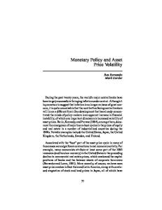
Percentage Difference from January 1994 !100 0 100 200

Figure 1: Selected Commodity Prices, 1994-2007

1994 1995 1996 1997 1998 1999 2000 2001 2002 2003 2004 2005 2006 2007 2008 Year Gold Price (log) Coffee Price (log)

Hog Price (log) Oil Price (log)

Notes: this graph shows daily data on (100 times) the log of prices of oil (Brent Crude), gold, coffee, and hogs. The series are normalized to be equal to zero at the beginning of 1994.

18

DEAN SCRIMGEOUR

Figure 2: Relationship between Commodity Prices on Event Days and Pre-Event Days Pre!Event Day

0 !10 !20

Change in Commodity Price

10

Event Day

!20

!10

0

10

20

!20

!10

0

10

20

Change in 3!month Eurodollar Futures Notes: this graph shows scatter plots of the percentage change in commodity prices against the change the three-month Eurodollar futures rate, on both pre-event days (left panel) and event days (right panel). The change in the interest rate is measured in basis points. The graph includes data from each commodity series used in the paper.

19

COMMODITY PRICES AND MONETARY POLICY

Figure 3: Dynamic Response of Commodity Prices to Monetary Policy Surprises

Estimated Response of Commodity Prices (Percent)

0.2

GSCI Futures Response VAR Response

0

-0.2

-0.4

-0.6

-0.8

-1 0

2

4 6 8 Months After Monetary Policy Surprise

10

12

Notes: this graph shows the estimated response over time of commodity prices to a monetary policy surprise using the Christiano, Eichenbaum and Evans (1999) VAR and GSCI commodity futures. The responses are shown with 95% confidence intervals. In the VAR, these are constructed using the 2.5 percentile and the 97.5 percentile of the distribution of responses in a Monte Carlo simulation where the parameter vector is drawn from a normal distribution centered on the VAR estimates, with the estimated parameter covariance matrix.

20

DEAN SCRIMGEOUR

Table 1: Variation of Commodity Prices and Covariation with Interest Rate Std. dev. of Commodity Price

Covariance with Policy Rate

Event Day

Pre-event

Event day

Pre-event

Gold

1.16

0.70

-2.62

-0.10

Aluminum

1.25

1.02

-1.82

0.04

Copper

1.48

1.30

-2.34

-0.36

Lead

1.75

1.59

-1.77

-0.26

Nickel

1.98

2.01

-3.01

-0.68

Platinum

1.33

1.14

-2.19

0.28

Silver

1.86

1.27

-4.02

0.39

Tin

1.27

1.26

-0.74

-0.19

Zinc

1.76

1.52

-2.40

-0.32

Cocoa

1.94

1.98

-2.60

0.84

Coffee

2.58

2.77

-1.99

-1.08

Cotton

1.52

1.47

-0.62

0.12

Wheat

1.82

1.30

-1.32

-0.52

Hogs

1.53

1.50

-1.65

0.06

Livestock

1.01

0.93

-0.98

0.05

Live Cattle

0.93

1.01

-0.93

0.16

Oil

2.77

2.39

-2.18

-0.26

Commodity

Notes: the change in the interest rate is measured in basis points. The change in commodity prices is measured in percentage points.

21

COMMODITY PRICES AND MONETARY POLICY

Table 2: Estimated Effects of Interest Rates on Commodity Prices Commodity All Commodities

All Metals

All Agricultural

All Vegetable

All Animal

Oil

Event Study

Rigobon-Sack

Excl. March 08

-5.55

-6.36

-4.52

(1.75)

(2.08)

(1.28)

-6.63

-7.49

-5.43

(2.24)

(2.69)

(2.18)

-4.09

-4.89

-3.19

(1.87)

(2.26)

(1.82)

-4.64

-5.04

-1.88

(2.69)

(3.33)

(2.35)

-3.37

-4.68

-4.95

(1.69)

(2.14)

(2.35)

-6.23

-6.68

-5.78

(3.68)

(4.75)

(4.47)

Notes: coefficients represent the estimated percentage responses of commodity prices to a one percentage point surprise in interest rates. Clustered standard errors in parentheses. (Clustering is at the level of date.) Standard errors for the effect on oil prices are White heteroskedasticity robust standard errors.

DEAN SCRIMGEOUR

22

Commodity

(1.90)

-2.11

(3.75)

-11.40

(3.29)

-6.13

(4.60)

-8.54

(3.12)

-5.30

(2.42)

-6.64

(2.04)

-5.15

(2.86)

-7.43

Study

Event

-7.20

(2.54)

-1.67

(4.79)

-15.10

(3.95)

-8.51

(5.73)

-8.18

(3.90)

-5.04

(3.02)

-6.68

(2.50)

-6.03

(3.45)

-8.54

Sack

Rigobon

(4.11)

-5.13

(2.78)

-2.06

(2.67)

-9.42

(2.90)

-5.05

(6.21)

-7.90

(3.47)

-2.83

(3.08)

-5.96

(2.50)

-5.20

(1.65)

-4.74

March 08

Excl.

(3.63)

-6.76

(2.76)

-3.21

(3.26)

-8.87

(2.67)

-5.22

(4.37)

-10.85

(3.67)

-2.83

(3.06)

-7.38

(2.53)

-6.28

(1.91)

-4.52

3SLS

Copper

Lead

Nickel

Platinum

Silver

Tin

Zinc

Cocoa

Commodity

-6.23

(1.59)

-2.64

(1.63)

-2.77

(2.40)

-4.68

(5.22)

-3.78

(3.73)

-1.77

(4.05)

-5.65

(2.82)

-7.35

Study

Event

(4.73)

-6.70

(2.06)

-3.81

(2.03)

-3.88

(3.12)

-6.54

(6.55)

-2.61

(4.56)

-2.72

(5.51)

-2.97

(5.00)

-11.93

Sack

Rigobon

(4.48)

-5.79

(2.08)

-3.73

(2.18)

-4.09

(3.39)

-7.23

(3.91)

1.670

(4.22)

0.12

(5.70)

-1.04

(4.09)

-8.32

March 08

Excl.

(5.78)

-4.32

(2.07)

-5.19

(2.15)

-5.17

(3.42)

-7.98

(3.35)

2.83

(3.31)

2.26

(5.76)

2.11

(4.27)

-7.81

3SLS

Oil

Live Cattle

Livestock

Hogs

Wheat

Cotton

Coffee

(3.68)

Table 3: Estimated Effects of Interest Rates on Commodity Prices

Gold

-6.78

(4.30)

Aluminum

(3.53 )

Notes: White heteroskedasticity robust standard errors in parentheses, except for 3SLS estimates, which are derived from a generalized least squares estimate of the system of equations. 3SLS estimates use data excluding March 2008 and also excluding 1994 since lead prices are unavailable for that year.

23

COMMODITY PRICES AND MONETARY POLICY

Table 4: Robustness Checks

Commodity All Commodities

All Metals

All Agricultural

All Vegetable

All Animal

Oil

With

With

Excluding

Kuttner

’89-’93

Testimonies

Reversals

Method

-6.68

-5.25

-6.94

-4.55

(2.39)

(1.89)

(2.76)

(1.27)

-7.94

-6.25

-6.71

-4.85

(2.98)

(2.46)

(3.49)

(1.72)

-3.91

-3.96

-7.27

-4.22

(2.76)

(2.00)

(2.67)

(1.31)

-2.86

-4.19

–7.94

-4.46

(4.22)

(2.89)

(3.96)

(1.81)

-5.32

-3.67

-6.39

-3.91

(2.69)

(1.90)

(2.81)

(1.38)

-14.41

-5.37

-6.68

-4.17

(7.92)

(5.01)

(6.17)

(3.40)

Notes: standard errors are clustered at the day level (or robust standard errors for oil).

24

DEAN SCRIMGEOUR

Table 5: Response of Commodity Price Futures Single Contract GSCI 1 Month

GSCI 2 Month

GSCI 3 Month

GSCI 4 Month

GSCI 5 Month

Equation

3SLS

-4.03

-4.03

(4.11)

(2.74)

-3.69

-3.69

(4.04)

(2.56)

-3.38

-3.38

(4.03)

(2.48)

-3.38

-3.38

(3.98)

(2.39)

-3.34

-3.34

(3.95)

(2.31)

Notes: this table presents estimates of the effect of monetary policy surprises on commodity futures contracts, using the Goldman-Sachs Commodity Index futures for one through five months. Robust standard errors for the first column, 3SLS standard errors for the second column.

COMMODITY PRICES AND MONETARY POLICY

25

Table 6: Commodity Prices and Changes in the Term Structure Commodity All Commodities

All Metals

All Agricultural

Two Year Rate

Long Forward Rate

-6.99

7.60

(2.30)

(5.68)

-7.47

9.23

(3.53)

(9.70)

-5.36

5.62

(1.77)

(4.86)

Notes: each row is a separate regression. Clustered standard errors in parentheses. (Clustering is at the level of the date.)

26

A

DEAN SCRIMGEOUR

Data Sources Table A.1: Commodity Prices Commodity

Series Name

Code

Gold

S&P GSCI Gold Spot

GSGCSPT

Aluminum

S&P GSCI Aluminum Spot

GSIASPT

Copper

S&P GSCI Copper Spot

GSICSPT

Lead

S&P GSCI Lead Spot

GSILSPT

Nickel

S&P GSCI Nickel Spot

GSIKSPT

Platinum

London Platinum Free Market $/Troy oz

PLATFRE

Silver

S&P GSCI Silver Spot

GSSISPT

Tin

LME-Tin 99.85% Cash U$/MT

LTICASH

Zinc

S&P GSCI Zinc Spot

GSIZSPT

Cocoa

S&P GSCI Cocoa Index Spot

GSCCSPT

Coffee

S&P GSCI Coffee Spot

GSKCSPT

Cotton

S&P GSCI Cotton Spot

GSCTSPT

Wheat

S&P GSCI Wheat(CBOT) Spot

GSWHSPT

Livestock

S&P GSCI Livestock Spot

GSLVSPT

Live Hogs

S&P GSCI Live Hogs Index Spot

GSLHSPT

Live Cattle

S&P GSCI Live Cattle Spot

GSLCSPT

Oil

Europe Brent Crude Spot FOB ($ per barrel)

RBRTE

GSCI 1 month

GSCI One Month Futures

GS1MSPT

GSCI 2 month

GSCI Two Month Futures

GS2MSPT

GSCI 3 month

GSCI Three Month Futures

GS3MSPT

GSCI 4 month

GSCI Four Month Futures

GS4MSPT

GSCI 5 month

GSCI Five Month Futures

GS5MSPT

Notes: All series in this table are taken from the Datastream database, except for the price of oil, which is taken from the U.S. Department of Energy’s Energy Information Administration.

27

COMMODITY PRICES AND MONETARY POLICY

Table A.2: Other Variables Variable

Source

Code

Three-Month Eurodollar Futures Rate

RC Research

ED

Federal Funds Futures Rate

RC Research

FF

Two-Year Treasury Constant Maturity

FRED

DGS2

Five-Year Treasury Constant Maturity

FRED

DGS5

Ten-Year Treasury Constant Maturity

FRED

DGS10