Co-occurrence of Transcription Factor Binding Sites Holger Klein Dezember 2009

Dissertation zur Erlangung des Grades eines Doktors der Naturwissenschaften (Dr. rer. nat.) am Fachbereich Mathematik und Informatik der Freien Universität Berlin

Gutachter: Prof. Dr. Martin Vingron Prof. Dr. Hanspeter Herzel

1. Referent: Prof. Dr. Martin Vingron 2. Referent: Prof. Dr. Hanspeter Herzel Tag der Promotion: 12. Mai 2010

Contents 1 Overview 1.1 Motivation and Thesis Structure . . . . . . . . . . . . . . . . . . . . . . . . 1.1.1 Publications . . . . . . . . . . . . . . . . . . . . . . . . . . . . . . . . 1.1.2 Acknowledgements . . . . . . . . . . . . . . . . . . . . . . . . . . . .

1 1 4 4

I

5

Background

2 Transcriptional Regulation 2.1 Molecular Biology of Gene Regulation . . . . . . . . . . . . . . . . . . 2.1.1 From DNA to Proteins . . . . . . . . . . . . . . . . . . . . . . . 2.1.2 Transcriptional Regulation . . . . . . . . . . . . . . . . . . . . . 2.2 Cooperation of Transcription Factors . . . . . . . . . . . . . . . . . . . 2.3 Experimental Methods . . . . . . . . . . . . . . . . . . . . . . . . . . . 2.3.1 Transcription Factor Binding Sites . . . . . . . . . . . . . . . . 2.3.2 Collections of Binding Sites and Regulatory Regions . . . . . . 2.3.3 Experimental Methods Protein-Protein and TF-TF Interactions 2.3.4 Collections of Protein and Transcription Factor Interactions . . 2.3.5 Summary . . . . . . . . . . . . . . . . . . . . . . . . . . . . . .

. . . . . . . . . .

. . . . . . . . . .

. . . . . . . . . .

7 7 7 9 12 14 14 18 19 20 21

3 Computational Prerequisites 3.1 Computational Prediction of Transcription Factor Binding Sites 3.1.1 Models . . . . . . . . . . . . . . . . . . . . . . . . . . . . 3.1.2 Application and Problems . . . . . . . . . . . . . . . . . 3.2 Computational Prediction of Transcription Factor Interactions . 3.2.1 Prediction of Protein-Protein Interactions . . . . . . . . 3.2.2 Prediction of Transcription Factor Interactions . . . . . 3.2.3 Summary . . . . . . . . . . . . . . . . . . . . . . . . . . 3.3 Computational Prediction of Regulatory Regions . . . . . . . . 3.3.1 Properties of Regulatory Regions . . . . . . . . . . . . . 3.3.2 Prediction of Regulatory Regions . . . . . . . . . . . . . 3.3.3 Summary . . . . . . . . . . . . . . . . . . . . . . . . . . 3.4 Similarity and Clustering of Position Weight Matrices . . . . . 3.5 Graph Theory and Graph Matching . . . . . . . . . . . . . . . 3.5.1 Graph Theory Definitions . . . . . . . . . . . . . . . . . 3.5.2 Graph Matching . . . . . . . . . . . . . . . . . . . . . . 3.5.3 Summary . . . . . . . . . . . . . . . . . . . . . . . . . . 3.6 Assessment of Results . . . . . . . . . . . . . . . . . . . . . . . 3.6.1 Receiver Operator Characteristics . . . . . . . . . . . . .

. . . . . . . . . . . . . . . . . .

. . . . . . . . . . . . . . . . . .

. . . . . . . . . . . . . . . . . .

23 23 23 30 31 31 32 36 37 37 37 41 41 42 42 43 47 47 47

. . . . . . . . . . . . . . . . . .

. . . . . . . . . . . . . . . . . .

. . . . . . . . . . . . . . . . . .

. . . . . . . . . . . . . . . . . .

i

Contents

II

Methods

4 A Co-Occurrence Score for the Prediction of Transcription Factor 4.1 Predicting TF interactions Based on TFBS Co-Occurrence . . . 4.1.1 Synopsis . . . . . . . . . . . . . . . . . . . . . . . . . . . 4.1.2 Counting Co-Occurring TFBSs . . . . . . . . . . . . . . 4.1.3 Counting Pairs in a Single Window . . . . . . . . . . . . 4.1.4 Counting Pairs in a Sliding Window . . . . . . . . . . . 4.1.5 Algorithm . . . . . . . . . . . . . . . . . . . . . . . . . . 4.1.6 Log-Odds Score and Expected Number of Pairs . . . . . 4.1.7 Summary . . . . . . . . . . . . . . . . . . . . . . . . . . 4.2 An Empirical PWM Similarity Measure . . . . . . . . . . . . . 4.3 Methods for Assessment of Results . . . . . . . . . . . . . . . . 4.3.1 Synopsis . . . . . . . . . . . . . . . . . . . . . . . . . . . 4.3.2 Relative Rank Sum of Interactions in Positive Set . . . . 4.3.3 Common Neighborhood Score . . . . . . . . . . . . . . .

51 Interactions . . . . . . . . . . . . . . . . . . . . . . . . . . . . . . . . . . . . . . . . . . . . . . . . . . . . . . . . . . . . . . . . . . . . . . . . . . . . . . . . . . . . . . . . . . .

5 Prediction of Regulatory Regions with Binding Site Graphs 5.1 Transcription Factor Binding Site Graphs . . . . . . . . . . . . . . . . 5.1.1 Synopsis . . . . . . . . . . . . . . . . . . . . . . . . . . . . . . . 5.1.2 Building Binding Site Graphs . . . . . . . . . . . . . . . . . . . 5.1.3 Calculation of Regulatory Potential from TFBS Graphs . . . . 5.1.4 Equivalence and Run-time Comparison of RMWM and RMBPM 5.1.5 Implementation . . . . . . . . . . . . . . . . . . . . . . . . . . . 5.1.6 Summary . . . . . . . . . . . . . . . . . . . . . . . . . . . . . .

. . . . . . .

. . . . . . .

. . . . . . .

III Applications 6 Prediction of Transcription Factor Interactions 6.1 Detection of Overrepresented PWM Pairs in Simulated Datasets 6.1.1 Synopsis . . . . . . . . . . . . . . . . . . . . . . . . . . . . 6.1.2 Simulation of a PWM Annotation Set . . . . . . . . . . . 6.1.3 Co-occurrence Scores for Artificially Enriched PWM Pairs 6.1.4 Summary . . . . . . . . . . . . . . . . . . . . . . . . . . . 6.2 Predicting Transcription Factor Interactions in Yeast . . . . . . . 6.2.1 Synopsis . . . . . . . . . . . . . . . . . . . . . . . . . . . . 6.2.2 Yeast TFBSs and Positive Interaction Set . . . . . . . . . 6.2.3 Known TF Interactions . . . . . . . . . . . . . . . . . . . 6.2.4 PWM Similarity for Yeast TFs . . . . . . . . . . . . . . . 6.2.5 Influence of Window Size, Scanning Threshold, and TFBS 6.2.6 Differences Between Homotypic and Heterotypic TF pairs 6.2.7 Over- and Underrepresented TF combinations . . . . . . . 6.2.8 Co-occurence Scores for a Clustered PWM set . . . . . . . 6.2.9 Summary . . . . . . . . . . . . . . . . . . . . . . . . . . . 6.3 Predicting Genome-wide TF Interactions in Human . . . . . . . . 6.3.1 Synopsis . . . . . . . . . . . . . . . . . . . . . . . . . . . . 6.3.2 Human TFBSs and Positive Interaction Set . . . . . . . .

ii

53 53 53 53 54 56 57 57 59 60 61 61 61 61 63 63 63 63 65 69 70 71

73 . . . . . . . . . . . . . . . . . . . . . . . . . . . . . . . . . . . . . . . . . . . . . . . . . . Overlap . . . . . . . . . . . . . . . . . . . . . . . . . . . . . . . . . . .

. . . . . . . . . . . . . . . . . .

75 75 75 75 77 78 79 79 79 79 80 81 84 86 88 89 90 90 90

Contents

6.4

6.5

6.3.3 PWM Similarity for Vertebrate TFs . . . . . . 6.3.4 Counting or Ignoring Overlapping TFBSs . . . 6.3.5 Potentially Interacting TFs . . . . . . . . . . . 6.3.6 Discussion . . . . . . . . . . . . . . . . . . . . . Prediction of TF Interactions in Specific Sequence Sets 6.4.1 Synopsis . . . . . . . . . . . . . . . . . . . . . . 6.4.2 Human Embryonic Kidney Cells . . . . . . . . 6.4.3 Tissue-specific Genes in Mouse . . . . . . . . . Comparing the Co-occurrence Score with a Theoretical 6.5.1 Synopsis . . . . . . . . . . . . . . . . . . . . . . 6.5.2 Dataset and Application of costat . . . . . . . . 6.5.3 Comparison of Performance . . . . . . . . . . .

. . . . . . . . . . . . . . . . . . . . . . . . . . . . . . . . . . . . . . . . Measure . . . . . . . . . . . . . . .

7 Predicting Regulatory Regions in Human 7.1 Calculation of Regulatory Potential for Known Regulatory 7.1.1 Synopsis . . . . . . . . . . . . . . . . . . . . . . . . 7.1.2 Murine Pax 6 . . . . . . . . . . . . . . . . . . . . . 7.1.3 Human Enhancers . . . . . . . . . . . . . . . . . . 7.2 Large Scale Assessment of Regulatory Potentials . . . . . 7.2.1 Synopsis . . . . . . . . . . . . . . . . . . . . . . . . 7.2.2 Sequence Sets . . . . . . . . . . . . . . . . . . . . . 7.2.3 Performance Assessment . . . . . . . . . . . . . . . 7.3 Discussion . . . . . . . . . . . . . . . . . . . . . . . . . . .

. . . . . . . . . . . .

. . . . . . . . . . . .

. . . . . . . . . . . .

. . . . . . . . . . . .

. . . . . . . . . . . .

. . . . . . . . . . . .

. . . . . . . . . . . .

91 92 98 101 102 102 102 106 109 109 109 110

Regions . . . . . . . . . . . . . . . . . . . . . . . . . . . . . . . . . . . . . . . .

. . . . . . . . .

. . . . . . . . .

. . . . . . . . .

. . . . . . . . .

. . . . . . . . .

111 111 111 111 113 117 117 117 118 121

IV Summary and Conclusions

125

8 Summary and Conclusions

127

Appendix

133

A German Summary

133

B Short Curriculum Vitae

137

C Ehrenwörtliche Erklärung

139

Bibliography

141

iii

iv

Chapter 1 Overview 1.1 Motivation and Thesis Structure Transcriptional Regulation Gene regulation deals with the processes, that enable an organism to create a large variety of cells and cell states from the same genome. A cell uses different genes under divergent conditions, for example in two phases of the cell cycle. In metazoan organisms completely different cell types, like a liver and a brain cell, are encoded in the same genome. However, the set of genes needed in both cases differs. A crucial step at which a cell regulates the production of proteins and other gene products is transcriptional regulation. The molecular machinery that transcribes the gene assembles at the transcriptional start site, the point from where an RNA copy of the gene is transcribed. The RNA is subsequently processed and often later on used as a blueprint for protein translation. The assembly of the transcriptional apparatus is governed by transcription factors: proteins that recognize and bind to the DNA and support tethering of the transcriptional apparatus to the transcriptional start site. We present a concise overview about the molecular biology of transcription in Section 2.1. To date the known target spectrum of transcription factors ranges from very specific factors with only a tiny number of targets under distinct conditions to ubiquituous factors, which influence the transcription of a large fraction of genes in a large variety of cell types and conditions. The estimated fraction of different transcription factors encoded in the human genome varies between 6 and 8%, leading to more than 2,500 different transcription factors [13]. The number of transcription factors expressed per human tissue is between 150 and 350 [342]. Transcription Factor Interactions and Regulatory Regions Aggregates of several transcription factors can act synergistically or antagonistically. Using combinations of transcription factors is beneficial to an organism, not only because of the many possible interactions which allow for fine-grained regulation, but also because a partial redundance of transription factors makes the transcriptional response more stable. The transcriptional network is dynamic, and the number of possible combinations of factor-factor and factor-DNA interactions in a complete organism is enormous due to the size of the genome, the number of different transcription factors, and the large number of different cell states and cell types. We summarize details about transcription factor interactions in Section 2.2. Transcription factors bind to two major classes of regulatory regions — promoters and enhancers. On the genomic sequence the promoters are located close to the regulated gene. Enhancers can be far away; in this case the interaction with the transcriptional machinery is

1

Chapter 1 Overview possible because of bending and looping of the DNA. The promoters harbor binding sites for general transcription factors which drive a low level of transcription, as well as for specific factors, that modulate the expression strength dependent on various factors. Enhancers usually influence specific expression. For properties of regulatory regions we refer the reader to Section 3.3.1. We present an overview of the large variety of experimental methods for the detection of transcription factor binding sites, transcription factor interactions and the detection of regulatory regions in Sections 2.3.1 and 2.3.3. Computational Methods Already the knowledge of the first binding motifs of transcription factors led researchers to search for more potential binding sites in other parts of the genome with in silico methods. Over time this lead to the development of copious methods for the prediction of transcription factor binding sites. A general problem of these methods lies in the nature of transcription factor binding sites. They are short and degenerate, which means that a high number of occurrences of a matching DNA motif is present by chance, rather than for a functional reason. We explain the general ideas and the problems that arise in Section 3.1. The prediction of transcription factor interactions is a difficult problem. Available methods make use of expression data, experimental binding data, overrepresented sequence motifs, or predicted transcription factor binding sites and apply a large variety of statistical methods. We summarize these methods in Section 3.2.2. Also for the prediction of regulatory regions one has the choice between many different tools. Partly they are sequence based only and deploy low level features like GC content or higher level features such as binding motifs. Other tools additionally utilise experimental data. We review various approaches in Section 3.3. Working Hypothesis The underlying assumption of the present work is, that in regulatory regions, binding sites of interacting transcription factors co-occur more often than expected by chance. The prediction of individual transcription factor binding sites is hampered by a large number of false positive results. Nevertheless we expect our assumption to be true also for predicted binding sites, even if the signal that emanates is weakened. To that end we develop two new methods, one for the prediction of transcription factor interactions, and one for the prediction of regulatory regions based on commonness of transcription factor binding site combinations. A Co-occurrence Score for Transcription Factor Binding Sites For the prediction of functional transcription factor interactions, we develop a counting method, which applies a sliding window over annotated transcription factor binding sites. The counting procedure is able to deal with overlapping windows, homotypic clusters, and overlapping binding sites. For the detection of overrepresented TFBS pairs, we calculate as a co-occurrence score the log odds score of observed over expected number TFBS pairs. We estimate the number

2

1.1 Motivation and Thesis Structure of expected pairs using a label permutation procedure with subsequent recountings. We describe our method in Section 4. We assess the counting procedure and the co-occurrence score on artificially generated datasets with defined number of co-occurrences in Section 6.1 and show, that the method is able to detect low TFBS pair enrichments. We apply the method to yeast regulatory regions in Section 6.2, and find that a large number of overrepresented TFBS pairs in fact belong to transcription factors known to interact. Moreover we examine the similarity of binding sites of interacting pairs and reasons for underrepresentation of TFBS pairs. In Section 6.5 we compare the co-occurrence score with the costat method by Pape et al. [253]. Subsequently we apply the method to vertebrate data in Chapter 6. Despite the much higher complexity of the regulatory network of vertebrates compared to yeast, we still find many known interactions among the top scoring pairs. This is the case for a genome wide study in human in Section 6.3, as well as for genes expressed in human embryonic kidney cells (Section 6.4.2), and tissue specific gene sets from mouse (Section 6.4.3).

Binding Site Graphs for the Prediction of Regulatory Regions Many tools for the prediction of regulatory regions explicitly or implicitly apply sequence properties like the GC content or the presence of CpG islands for the detection of regulatory regions. We aim to design a method, which is less dependent on low level features and hence makes use of the knowledge about over- and underrepresented TFBS pairs in known regulatory regions to measure the regulatory potential. We represent the predicted binding sites in a sequence to be characterised as the vertices in a graph. Subsequent assignment of co-occurrence scores as edge weights for all vertex pairs leads to a binding site graph. The co-occurrence scores originate from known regulatory regions and are calculated with the method from Section 4. Using this graph, we now can calculate various edge-weight based scores for the input sequence, which we call regulatory potentials and which represent the level of abundance of transcription factor combinations typical for regulatory regions. We present our approach in Chapter 5. In Chapter 7 we apply the methods to known regulatory regions. We show the performance of one of the scores on the well examined regulatory regions of the murine PAX6 gene and known human enhancer regions from the VISTA set. In Section 7.2 we assess the reliability of our method for genome-wide prediction of regulatory regions based on test sets, consisting of promoter and enhancer regions as positive sets and an artificial, shuffled sequence set and an intergenic set as negative sets. We find, that although the biggest factor playing a role in the prediction of regulatory function again is the GC content of a candidate sequence, our method should be used to filter out false positive predictions of regulatory function based on GC content. In Chapter 8 we summarize and discuss our findings.

3

Chapter 1 Overview

1.1.1 Publications Some of the work presented in this thesis has been published in the paper “Using Transcription Factor Binding Site Co-Occurrence to Predict Regulatory Regions”, Klein & Vingron, Genome Informatics, 2007. The costat method, to which we compare our co-occurrence score was published in the paper “Statistical detection of co-operative transcription factors with similarity adjustment.”, Pape, Klein, Vingron, Bioinformatics, 2009.

1.1.2 Acknowledgements During my time in the gene regulation group in the department for computational molecular biology at the Max Planck Institute for Molecular Genetics, I enjoyed an intellectually stimulating and friendly environment. First of all I want to thank Martin Vingron for the opportunity to work on an interesting topic in his group, and for the ideas and continuous support that I received from him in the time that I spent at the MPI. Moreover, I would like to acknowledge the International Research and Training Group (IRTG), the PIs and fellows of which provided an additional inspiring forum to discuss ideas related to this thesis. I spent two months in Zhiping Weng’s lab, during which I received a lot of input from Zhiping and other group members. Apart from thanking all members of the department, I would like to individually mention a number of people for longer discussions related to my work, providing data, and/or proofreading of the present manuscript: Hannes Luz, Hugues Richard, Sarah Behrens, Utz Pape, Marcel Schulz, Sean O’Keefe, Abha Singh Bais, Steffen Grossmann, Stefan Röpcke, HansJörg Warnatz, Helge Roider, Ho-Ryun Chung, Christoph Dieterich, Szymon Kiełbasa. I enjoyed sharing my office with Christoph and Szymon. The scientific and professional interactions within the group and the institute often evolved to friendship. I would not want to miss that. I would like to acknowledge my parents Birgid and Hans-Josef Klein for their ongoing support and encouragement (not only during the time of my thesis). Lastly, I want to thank Vesna for her patience and support.

4

Part I

Background

5

Chapter 2 Transcriptional Regulation The focus of the present work lies on the prediction of transcription factor interactions and their use for the prediction of regulatory regions. We will begin this chapter with a short summary of the biological context of eukaryotic gene regulation. We will then shift the focus towards transcription factors and their co-operation. Subsequently we will provide an overview of the most important experimental methods for the detection of transcription factor binding, transcription factor co-operation, and regulatory regions. Here we can only give a short introduction into the topics. For more details we refer to textbooks like Alberts et al. [8].

2.1 Molecular Biology of Gene Regulation 2.1.1 From DNA to Proteins The Structure of DNA The genetic information of a living organism is stored in the deoxyribonucleic acid (DNA). The DNA consists of a chain of nucleotides; sugar molecules combined with one of the bases adenine (A), cytosine (C), guanine (G), and thymine (T). Combined via phosphodiester bonds, the sugar molecules form the backbone of the DNA. Chargaff [57] found that the bases C and G as well as A and T form pairs and hence occur in equal fractions in the DNA. The base pairing leads to the well-known double-helix structure of the DNA, published by Watson and Crick [353]. It consists of two anti-parallel, complementary strands, the direction of which is defined by the position of the phosphodiester bonds in the sugar molecules: the bonds connect the 5’ carbon of one deoxyribose to the 3’ carbon of the next. The synthesis and processing of DNA only takes place in the direction from the 5’ end to 3’ end. This directionality also defines the terms upstream (5’) and downstream (3’). Figure 2.1 shows the chemical structure of the four bases and the pairing of bases. Cells of eukaryotic organisms, unlike bacteria, contain nuclei which harbour the chromosomes. The chromosomes are structures that consist of the double stranded DNA and accessory structural proteins. The DNA is wound around the nucleosomes, each of which consists of a histone octamer. One loop of the DNA around a nucleosome has the length of 146 base pairs (bp). Figure 2.2 shows different packing levels of the DNA. The DNA is only in the fully condensed state when entering the process of cell division. Otherwise the condensation state can either be active euchromatin, or silent heterochromatin, meaning that the DNA is easily

7

Chapter 2 Transcriptional Regulation

Figure 2.1: Building blocks if the DNA and base pairing. Guanine / Cytosine pairs are connected by three, Adenine / Thymine pairs by two hydrogen bonds. Image reproduced with permission from http://www.accessexcellence.org/, National Health Museum, USA

accessible for other proteins or not.

Genes, Transcription and Translation The classical definition of a gene is a stretch of DNA, that encodes functional cellular components like proteins. In a process called transcription, the enzyme RNA polymerase transcribes the DNA of a gene into ribonucleic acid (RNA). The RNA is a linear bio-polymer, similar to the DNA, but consists only of a single strand, and with uracil (U) instead of the thymine in the DNA (Figure 2.1). The RNA plays a role in direct catalysis of metabolic processes and as a structural component in RNA protein complexes, and on the other hand as messenger RNA (mRNA) as a template for the production of proteins. For the production of proteins the first step is the splicing of the primary transcript. The introns are removed, resulting in the mature mRNA, which only consists of the exons, combined to the open reading frame (ORF), and 5’ and 3’ untranslated regions (UTR). By variation of exon usage, splicing can lead to different splice forms or alternative transcripts, finally resulting in different protein products from the same gene. Subsequently the mature mRNA is transported out of the cell nucleus to the ribosomes, in which translation to a chain of amino acids based on the genetic code takes place. In human, roughly 1.5% of the complete genome are exonic sequences. Figure 2.3 exemplifies a eukaryotic gene with the transcriptional unit containing exons, introns, and UTR. The flow of information from DNA to RNA to protein is commonly known as the central dogma of molecular biology, a term coined by Crick [70].

8

2.1 Molecular Biology of Gene Regulation

Figure 2.2: Structural organization of the genome. The nucleus in the cell contains the chromosomes. The chromosomes consist of identical sister chromatids. The DNA is wound around the nucleosomes, which are built from eight histone molecules (octamer). Image reproduced with permission from http://www.genome.gov/, National Human Genome Research Institute, USA

2.1.2 Transcriptional Regulation An organism requires the various genes in different amounts and under different conditions. Thus the creation of gene products is controlled at all levels, from chromatin modifications over transcriptional regulation to post-translational modifications and protein degradation. In the following, we will focus on transcriptional regulation, since this is the most important aspect with respect to this thesis.

Regulatory Regions and the Transcriptional Machinery A part of a gene not mentioned before is the promoter. It contains the information needed for the activation or repression of gene [256, 309] . In eukaryotes, the transcription of a genes starts with the assembly of the pre-initiation complex on the promoter. The pre-initiation complex contains 10 to 12 proteins, among them the general transcription factors [194, 246] and one of three different RNA polymerases, in case of protein coding genes RNA polymerase II. A common definition for the promoter is the region upstream of the transcriptional start site (TSS). The promoter is divided into two parts: the core or basal promoter at roughly -35bp relative to the TSS, which the aforementioned transcriptional apparatus binds to. For a part of the genes, it contains the TATA box, a sequence motif which the TATA-binding protein

9

Chapter 2 Transcriptional Regulation

Figure 2.3: Structural organization of a eukaryotic gene. The promoter contains several cisregulatory modules. The transcriptional unit consists of exons, introns, and untranslated regions. Image reproduced from Wray et al. [361].

(TBP) binds to [202]. The proximal promoter ranges up to a few hundred bp upstream of the TSS. It contains binding sites for for other, mostly sequence-specific TFs, needed for the activation or repression of the regulated gene in various conditions [196]. Another type of genomic region that influences the transcription is the enhancer [177]. It also harbours binding sites for sequence-specific TFs, but can be far away from the TSS, up to 100,000bps [150] or even 1,000,000bps away [259, 179]. Nevertheless the TFs that bind to enhancers interact with the transcriptional apparatus at the promoter by looping of the DNA. The TFs, that are part of the transcriptional apparatus activate unspecific expression on a low level. For higher expression levels as well as specific spatial or temporal regulation of gene expression, TFs that bind to the proximal promoter and enhancers play a role. Figure 2.4 illustrates the binding of the transcriptional machinery to the promoter and the interaction with enhancer modules.

Figure 2.4: Transcriptional regulation. Several general transcription factors bind to the basal promoter, among them the TATA binding protein TBP and other TATA associated factors (TAF), to form the preinitiation complex. The regulatory regions contain several cisregulatory modules, to which combinations of TFs bind. Image reproduced Wray et al. [361]

For an extensive review of regulatory elements see Maston et al. [217].

Number of Transcription Factors The human body consists of more than 200 different cell types [337] and an estimated number of 20,000-25,000 different genes spread over a genome of more than 3,000,000,000bps [65], and a part of the tissues requires tight spatial

10

2.1 Molecular Biology of Gene Regulation and temporal regulation of gene expression. Only a subset of the genes in a eukaryotic cell are expressed at any given time, and the proportion and amount changes during life cycle, among cell types, in response to external conditions [161, 356, 11]. Hence it is not a surprise that eukaryotic organisms have a many different TFs. Nimwegen [236] finds that large genomes tend to have more TFs. The number of genes with known DNA-binding domains in baker’s yeast Saccharomyces cerevisiae is 245, which corresponds to 3.9% of the genes. In human there are 2604 genes with known DNA-binding domains, amounting to roughly 8.1% of all genes [13]. Vaquerizas et al. [342] estimate that roughly 6% of human genes are TFs, with an upper bound of 8.2%. In human, between 150 and 350 different TFs are expressed per tissue. On average 6% of expressed genes in a tissue are TFs [342]. The expression patterns of TFs themselves are highly complex and expression takes place in distinct domains [75, 76].

Transcription Factor Binding Up to now, eight different structural groups of transcription factors are known. They belong to 54 different structural families [207] and can draw on 12-15 different DNA-binding domains [143]. The transcription factor binding sites (TFBSs) on which the TFs interact with the DNA are typically short and degenerate. The length of the DNA region with physical contact with a TF is usually between 10 and 20bps with a core of five to eight bps which are required to contain specific bases. The distance between TFBSs is constrained for sterical reasons [12]. A typical promoter has an occupancy of TF binding of 10 to 20% of its sequence.

Modulation of Transcription Factor Activity An organism has a number of possibilities to influence the activity of a TF. An obvious way is to change the expression of the factor itself on the level of transcription as well as on the level of translation [1]. Formation of dimers, presence of cofactors, as well as post-translational modifications are another option. On the other hand modifications of the DNA allow the modulation of TF binding to the DNA: Histone modifications like (de-)acetylation or (de-)methylation of the side chains lead to a higher or lower compaction of the DNA-histone complexes, hence increasing or decreasing the accessibility of regulatory regions for the transcriptional machinery [113]. The most common modification of the DNA molecule itself is the DNA methylation, specifically of the cytosine in CG dinucleotides (often referred to as CpG, with p representing the phosphodiester bond). Cytosines in CpG dinucleotides are methylated by DNA methyltransferases to form 5-methyl-cytosine. Methyl-cytosines are prone to transition mutation to a thymine [288], hence the CG dinucleotide is rare in mammalian genomes. Evolutionary constraints lead to higher amounts of CG dinucleotides in regulatory regions, often occurring in clusters called CpG islands. The organism can selectively methylate and demethylate CG dinucleotides. A methylated CG dinucleotide in a regulatory region prevents binding of TFs, which results in inhibition of expression. The promoters of roughly 40% of mammalian genes contain CpG islands [101]. The original definition for a CpG island requires a size of over 200bps, a GC percentage of more than 50%, and an observed over expected CpG ratio above 60% [120]. Saxonov et al. [287] identified two classes of human promoters, based on their CpG observed over expected ratio, with a tendency of the high CpG promoters belonging to “house keeping”

11

Chapter 2 Transcriptional Regulation genes, that are ubiquitously expressed and the low CpG promoters belonging to specifically expressed genes.

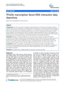
2.2 Cooperation of Transcription Factors Proteins fulfill their function in the organism in cooperation with other proteins. Estimated numbers of interactions for E. Coli proteins are within a range of two to ten [213], in yeast the average number of interactions is five [129]. This is also true for TFs: although a variety of factors is available in a typical eukaryotic cell, the complex expression patterns mentioned in the previous section require combinations of TFs to achieve specific regulation. In eukaryotes transcription factors are usually part of bigger complexes consisting of several factors and co-factors. Normally it is not a single transcription factor which regulates the spatial and temporal expression patterns of a gene, but combinations of transcription factors. A common transcription factor is organized in a modular fashion and consists of at least one DNA-binding domain and a trans-activating or interaction domain, which enables the factor to interact with other transcription factors or co-factors. Some transcription factors carry other domains, like ligand-binding domains in the case of hormone-receptors, which upon binding of a ligand modulate the activity of a factor. The TFs involved in such a complex bind the DNA in sterical proximity, hence the respective transcription factor binding sites lie close to each other on the DNA sequence. The footprint of a transcription factor complex is a cluster of TFBSs commonly called a cis-regulatory module (CRM). This concept goes back to the group of Eric Davidson [180, 372, 24]. For metazoans a typical CRM consists of 10 to 50 binding sites for at least three to 15 different sequence-specific transcription factors spread over up to 500bp [361, 197, 12]. Balmer and Blomhoff [24] estimate the mean length of a CRM to 600bps, with a mean of 24.5 TFBSs [24]. Sometimes multiple similar binding sites increase the sensitivity for a TF [150], lead to a more robust transcriptional response [304], play a role in the activation of morphogen TFs in response to low local TF concentration [133], or simply lead to the binding of a homo-oligomer of the TF (e.g. p53, or NF-κB ). These homotypic clusters exist in various organisms, for example yeast [348], Drosophila melanogaster [201, 12], and human [375]. Some transcription factors have well known interaction partners. We call the type of interaction homotypic if the TF interacts with a second factor of the same type. The factor GATA-1 is a well known example displaying homotypic interactions [72]. The interaction is called heterotypic if the factor interacts with a factor of another type. Moreover, DNA-binding transcription factors can interact with other DNA-binding factors in an indirect way by mediation of co-factors. Often a given transcription factor can interact with a variety of other factors. Replacement of a TF in a complex can but does not need to change the function of the whole complex. A variety of known cis-regulatory modules can be accessed from the TRANSCompel database [173]. TFs can act together in synergistic or antagonistic fashion [12, 104, 372]. A well studied example of a complex of transcription factors acting together synergistically is the combination of nuclear factor of activated T cells (NFAT) belonging to the REL family of factors and the AP-1 hetero-dimer, which itself consists of the two factors Fos and Jun. The complex activates the transcription of many genes playing a role in immune response. The crystal structure of the complex is shown in Figure 2.5. NFAT and AP-1 directly interact with

12

2.2 Cooperation of Transcription Factors each other, hence the respective binding sites lie directly next to each other on the DNA sequence [59].

Figure 2.5: Crystal structure of the NFAT – AP-1 complex binding to a DNA fragment from the interleukin-2 (IL-2) promoter (PDB id 1A02 [59], image created with VMD [155]). NFAT (green) belongs to the Rel-family transcription factors and contains a Rel homology region (RHR). AP-1 is a heterodimer leucine zipper consisting of the factors JUN (orange) and FOS (yellow). The DNA sequence (strands in blue and red) which is bound contains a binding site for NFAT (GGAAA) and a binding site for AP-1 (TGTTTCA) divided by a two base long spacer sequence (TT). NFAT and AP-1 have a large contact surface with mostly polar interactions. Chen et al. [59] expect that the complex shown here is part of a larger complex containing more partners.

Another immune-response related example for interacting transcription factors are ATF3 from the CREB/ATF family of transcription factors and the nuclear factor NF-κ B [124]. The binding of ATF3 and its interaction partners was shown to repress transcription of cytokine genes. Like NFAT, NF-κ B contains a REL domain needed for interaction with other factors. Gilchrist et al. [124] found the TFBSs for the combination of ATF3 and NF-κ B to lie close to each other in respective targets. Moreover they discovered a direct interaction of the factors - as well as interactions of ATF3 with the aforementioned Jun and Fos.

13

Chapter 2 Transcriptional Regulation Implications of Combinatorial Regulation There are several salient advantages of combinatorial regulation. Due to interactions between two or more factors, an organism can realize a wide variety of transcriptional responses already with a small number of different transcription factors. Combinatorial regulation allows for a much higher number of distinct expression states than the number of transcription factors present in an organism [169]. Moreover simple exchange of single components can modulate the function that a complex fulfills: this way the expression of target genes can vary from cell type to cell type or between different conditions. If a TF in a complex can be replaced without a change in the transcriptional response, the regulatory system gains robustness [335]. Also TFs which themselves do not have a clear DNA binding preference might “inherit” specificity from a more specific interaction partner. For the factors from the bZIP family including for example Jun, Fos, and CREB/ATF, Ryseck and Bravo [283] showed differences in the binding specificity depending on the interaction partners [283]. The homeodomain TF pair MATa1 / MATα 2 plays a role in the yeast cell cycle and its combined DNA affinity is much higher than that of the individual TFs [199]. Other homeodomain TFs also change their binding specificity depending on co-factors [344]. This is in accordance with the finding of Bilu and Barkai [36], that regions which bind many transcription factors tend to have shorter and fuzzier TFBSs than sites which bind only few TFs.

2.3 Experimental Methods 2.3.1 Transcription Factor Binding Sites Several experimental methods for the detection of transcription factor binding sites have been developed over the years. The methods can be divided into time consuming low throughput methods, which can precisely localize a transcription factor binding site and high throughput methods which require a subsequent computational analysis [96]. Moreover the methods differ depending on whether the factor for which binding sites are sought is known or not. Regulatory regions are the parts of the genome to which transcription factors bind to influence transcription of genes. Thus the experimental methods used for the detection of regulatory regions largely overlap with the ones used for the detection of transcription factor binding sites. In the following we give an overview of the most important techniques. DNase I Hypersensitivity In regions with an open chromatin structure the DNA is accessible for other proteins like transcription factors or nucleases such as DNase I. This can be exploited to detect regions which are sensitive for cleavage by DNase I and thus are also potentially accessible for transcription factors [123]. The state of the chromatin depends on factors such as the cell type, the developmental stage or the environment normally leading to different DNase I hypersensitive regions. The genome contains large scale DNase hypersensitive regions with sizes between 10 and 100 kilobases [193] but also local hypersensitive regions with sizes between 100 and 400bp [130]. Hypersensitivity in non coding portions of the genome can be used as a marker for transcription factor binding [56]. While the above mentioned methods are considered to be low throughput there are high

14

2.3 Experimental Methods throughput methods, which in their results differ in the resolution. Indirect end-labelling provides a resolution of ca. 500bp [363], while quantitative PCR methods provide a resolution on nucleotide level [366, 220]. Other high throughput methods include quantitative chromatin profiling [86], massive parallel signature sequencing [69] and using tiling arrays for the determination of nucleosome positions [371]. The method can be applied for genome wide detection of potential regulatory regions. Promoter Analysis Gene expression assays measure the amount of a reporter protein in response to changes in cis-regulatory elements in the respective upstream promoter. The most common reporter constructs use luciferase, a gene whose product causes bioluminiscence [79], and green fluorescent protein (GFP) from jellyfish, which displays fluorescence when exposed to ultraviolet light [336]. The bioluminescence and the fluorescence allow for simple methods to measure the expression levels of the reporter genes. After incorporation of the reporter into a plasmid, the plasmid is used to transfect a cell. The expression level of the reporter depends on the promoter sequence upstream of the reporter gene. Transcription factors in the cell bind to the promoter and influence the expression of the reporter. Mutations of sequence positions which play a role in the binding of a factor influence the expression level of the reporter gene, thus allowing the identification of transcription factor binding sites. Different groups adapted the method for high throughput usage by alternative transfection methods such as lipofection [323], coinjection [232], and nucleofection [303]. Mobility Shift Assays In this type of assay one applies an electrical potential to a polyacrylamide gel which contains DNA and transcription factors. The voltage causes a movement of the molecules in the gel, which depends on the size of the molecules. DNA bound by a transcription factor moves slower than unbound DNA. Because the DNA is radio-nucleotide labelled, bands in the gel show up and it is possible to read out the distance that a molecule has travelled. The electric mobility shift assay (EMSA) was one of the first methods to investigate proteinDNA interactions [110, 121, 145]. The assay uses a transcription factor and fragments of DNA of roughly 25bp. If the DNA is not bound by the transcription factor, the gel contains two bands, one for the unbound DNA and one for the transcription factor. If the transcription factor binds the DNA, one expects a third band for a molecule of higher weight, the complex of the DNA bound by the transcription factor. Using different DNA sequences allows for scrutiny of the specificity of the transcription factor [167]. A disadvantage of the method is the potential detection of non-specific DNA-protein interactions [183]. An alternative method combines the DNA-protein binding reaction of EMSA with the cleavage reaction of DNase I. DNase I footprinting uses the fact that DNase I can not cleave transcription factor-bound DNA. Visualization of the bands for the radio-nucleotide labelled DNA fragments shows regions devoid of bands representing binding sites in a semicontinuous ladder of bands. DNA sequences used in a footprinting experiment have a length of up to 500bp, resulting in the possibility to localize several transcription factor binding sites at once [116]. Newer methods make use of fluorescent labels [243] instead of radio-nucleotide labelling. Chemical cleavage is an alternative to the usage of nucleases. This solves enzyme

15

Chapter 2 Transcriptional Regulation specific problems [89], but does not tackle the issue of unspecific DNA-protein interactions [183].

Nitrocellulose Binding Assay An early method to measure binding of a transcription factor to DNA is the nitrocellulose binding assay [360]. The basis of the assay is negatively charged nitrocellulose paper. Proteins with a net-positive charge bind to the nitrocellulose while negatively charged DNA does not. Washing removes the non-bound DNA from the nitrocellulose filter. The DNA still present is considered to be bound to the transcription factor. Afterwards the bound DNA is eluted by a denaturing enzyme and analyzed in a subsequent gel electrophoresis. Using this assay it is not possible to detect the binding site on the DNA itself. Nowadays the assay is rarely used and has been replaced by a variety of other methods.

NMR and X-ray structures X-ray and NMR spectroscopy resolves the structure of a transcription factor bound to DNA. This time-consuming procedure is carried out for a small number of factors. An example is the X-ray structure of the heterodimer consisting of NFAT and AP-1 together with a piece of DNA [59]. Using structures it is possible to not only investigate the sequence of a transcription factor binding site but also if the factor bends or torts the DNA. Apart from requiring a lot of time to obtain structures it is impossible to crystallize some proteins. Another drawback is that one usually can only observe a single specific binding site, which might not be representative. Luscombe et al. [207] present an overview of available structures of transcription factors in the PDB database.

SELEX and CAST SELEX (Selective Evolution of Ligands by Exponential Enrichment [242, 339, 109]) and CAST (Cyclic Amplification and Selection of Targets [362]) are both in vitro approaches for the detection of the binding specificity for a known transcription factor. Both screen large pools of short, random oligonucleotides and amplify sequences that bind to the transcription factor in several rounds. Recent in vitro approaches include DIP-ChIP (DNA immunoprecipitation with microarray detection) [204] and double-stranded DNA microarray chips [51, 16, 230].

Chromatin Immunoprecipitation Assays Chromatin Immunoprecipitation (ChIP) is a method to experimentally determine regions of the genome to which a specific transcription factor binds in vivo [313, 45, 245]. Formaldehyde or another cross-linking agent induce the formation of covalent bonds between the transcription factor and the DNA. Subsequently sonication causes cleavage of the DNA into pieces of a size of 100 to 500bp. A specific antibody containing an anchor tags the transcription factor. The antibody allows for retrieval by precipitation of the parts of the DNA cross-linked to the transcription factor. After reversal of the cross-linking process the analysis of the precipitated DNA results in the regions of the genome to which the factor in question bound. The main bottleneck for the ChIP method is the limited availability of transcription factor specific antibodies. A problem of the method is the detection of indirect contacts due to protein-protein interactions.

16

2.3 Experimental Methods ChIP Amplification The analysis for the DNA fragments retrieved from the chromatin immunoprecipitation are determined by PCR and followed by sequencing. The preparation of primers for the PCR requires previous knowledge about the genomic region where the transcription factor is supposed to bind. The precise binding location within the genomic fragments can not be determined by sequencing only. Combining the chromatin immunoprecipitation with DNase protection and cleavage allows for to identify the specific binding site [168]. ChIP-Chip and ChIP-Seq ChIP-chip and ChIP-seq both combine chromatin immunoprecipitation with a high throughput technology which permit genome wide analyses of ChIP results. In ChIP-chip one identifies the precipitated DNA by microarray analysis [275, 161, 139]. Hybridization of the DNA fragments to microarray probes and subsequent readout delivers information about enrichment of sequences bound to the transcription factor. Early applications of the method used cDNA microarrays [275], later followed by 50mer oligonucleotide tiling arrays [178]. ChIP-chip methods were applied to a wide variety of transcription factors, genomic regions, cell types and organisms, for example intergenic regions in yeast [275], putative promoter regions in human [200, 239], human CpG island associated promoters [354], genome wide promoters in fibroblasts [178]. Subsequently the statistical analysis of spot intensities is crucial for the determination of most probable binding regions of the transcription factor in question. Buck and Lieb [49] summarize common methods. A more recent alternative to the identification of precipitated DNA using microarray chips is next-generation sequencing. Here the DNA is sequenced-by-synthesis in parallel after being attached to a surface. Pyrosequencing [215], usage of fluorescent reversible terminator deoxyribonucleotides [30, 31], or sequential ligations [300] permit fast and accurate sequencing of large amounts of DNA at the same time. A successive mapping of the TF bound DNA sequences to the genome is necessary. For a review of next-generation sequencing technologies see [299]. Recent examples for ChIP-seq applications are the determination of STAT1 binding sites [277] and the investigation of nucleosome positioning in human promoters [291]. While requiring a high quality reference genome sequence, the advantage of ChIP-seq methods over ChIP-chip is that the accuracy of the result is not limited by the location of probes in the genome. The resolution of binding site localization is in the order of tens of base pairs. The procedures require less material and less replicate experiments, and the results are highly similar to the ones of ChIP chip [214]. Detection of Transcriptional Start Sites The transcriptional start site (TSS) can be used to define putative promoter regions of genes. Cap Analysis of Gene Expression (CAGE) [301] is the most common method for the determination of TSSs. The CAGE method consists of capturing, sequencing, and mapping the 5’ end of mRNAs in a biological sample to a reference genomic sequence, leading to TSS locations. The TSS then defines putative promoter regions in the vicinity. Depending on the organism, various regions around transcriptional start sites are considered to comprise promoter regions. While there are reports of regulatory interactions between regulatory elements as far away from the TSS as 1Mbp [259, 179] or 100kbp [150], the majority of interactions with the basal transcription machinery seems to happen in a short range on the core promoter. For Homo sapiens Qian et al. [268] use a region of -1000 to 0 bp relative to the TSS, since

17

Chapter 2 Transcriptional Regulation it was claimed to contain the highest density of known binding sites [369]. Xie et al. [365] find the the highest density of evolutionarily conserved motifs in the region between -500 and +200bp relative to the TSS. The ENCODE project found that 67% of real TFBSs are located within 2.5kb of TSS [63]. Tabach et al. [328] show that the region with the highest abundance of location-specific TFBSs in human and mouse extends from -200 to +100bp relative to the TSS[328]. The concentration of functional and conserved TFBSs close to the TSS suggests a limitation of the extracted sequence region to a few hundred base pairs to 1kbp to limit the fraction of false positive TFBS predictions. Summary A plethora of experimental methods are available for the examination of transcription factor binding specificities and the localization of the respective sites. For a known transcription factor, technologies like SELEX or CAST can elucidate the binding specificity, while ChIP combined with a consecutive analysis of bound DNA produces the location of the binding sites. Elaborate methods involving the resolution of transcription factor structures are time-consuming, but carried out in cases of specific interest. If the transcription factor in question is not yet known, methods like DNase I hypersensitivity generate possible genome wide candidate regions for regulatory activity. The combination of EMSA and DNase I also resolves binding site locations. Reporter constructs make the examination of binding sites for known or unknown factors possible for smaller numbers of candidate sequences. In recent time large scale approaches using ChIP combined with modern sequencing technologies became feasible and prevalent. Detection of the transcriptional start site supports the definition of putative promoters in the vicinity of the TSS.

2.3.2 Collections of Binding Sites and Regulatory Regions Transcription Factor Binding Sites Two bigger collections of transcription factor binding sites exist. At this time the TRANSFAC database [219] contains 885 different binding site profiles (version 2009.1) of different quality, many of which stem from the same factor. JASPAR [346] comprises a smaller, but non-redundant set of profiles (123 matrices in version 3.0). Various other projects collect profiles for specific organisms, like yeast [374, 142, 208], or different bacteria [210, 284]. The recently started PAZAR project [264] aims to unify various collections of experimentally determined transcription factor binding sites in an open-source and open-access fashion.

Collections of Regulatory Regions The Saccharomyces cerevisiae promoter database (SCPD) [374] annotates regulatory regions in yeast. New experimental data from genomewide detection of DNase I hypersensitive regions in yeast provide a more complete and detailed picture of regulatory regions in yeast [35, 98]. One of the first collections of regulatory regions for higher organisms was the eukaryotic promoter database EPD. It started as a manually curated compilation of published promoter sequences [48] in 1986. The most recent version 100 [292] contains 4809 promoter sequences from various species, the majority from mammalia. The database of transcriptional start sites (DBTSS) [349] is a collection of experimentally determined 5’-end sequences of full-length cDNAs for Homo sapiens and Mus musculus. The current release 6.0.1 contains approximately 19 million 5’-end sequences derived from

18

2.3 Experimental Methods next-generation sequencing mapped to the human genome. Another source of transcriptional start sites is the EnsEMBL database [153], which annotates transcripts for a large variety of organisms based on evidence from the EMBL nucleotide sequence database [62], the protein sequence collection UniProtKB [66], and the manually annotated mRNAs and proteins from NCBI RefSeq [355]. The FANTOM project provides collections of full-length cDNA sequences based on the CAGE technology [170, 64].

2.3.3 Experimental Methods Protein-Protein and TF-TF Interactions Most experimental methods which provide information about transcription factor interactions are not specific for transcription factors, but are designed to detect general proteinprotein interactions (PPI). There are approaches to screen PPIs and others to verify PPIs. Some methods detect interactions in vivo, others in vitro. Because of the normally low expression levels of transcription factors themselves and of methodological reasons the elucidation of interactons between transcription factors is generally more difficult than between other proteins. In the following we present the main approaches.

Screening Methods In the yeast two-hybrid (Y2H ) experiment [106] the coding sequences of the DNA-binding domain and the activation domain of a transcription factor, often GAL4, are separately fused with a bait protein and potential interaction partners as prey proteins. If the bait and a prey protein interact, the separated domains come together and activate the transcription of a reporter gene which is expressed in case of an interaction. The method functions in quasi in vivo circumstances. The method has been fully automated, is highly sensitive but has many false positive predictions. Using Y2H for the elucidation of TF interactions is problematic, because the domains fused to bait and prey proteins possibly interact with other domains then their original partner, leading to less reliable results. Yeast two-hybrid screens exist for several organisms, for example for yeast [341, 159] or for human [320, 282]. Protein cross-linking works by forming covalent cross-links between lysine residues of proteins and can detect weak interactions [258]. Neighbouring proteins from a complex can lead to false-positive predictions. Cross-linking can be performed in vitro and in vivo. Tandem Affinity Purification (TAP) [276] is a method to rapidly purify protein complexes under natural conditions such that one can identify the components of a complex using mass spectrometry. It comprises of a two-step purification after fusing a TAP tag with a target protein. TAP is not limited to binary interactions, but in some setups the false-negatives caused by low abundance and transient interactions are problematic. High-Throughput Mass Spectrometric Protein Complex Identification (HMS-PCI) directly identifies protein complexes by mass-spectrometry [149]. A one-step immuno-affinity purification based on epitope tags allows to capture bait proteins, which are subsequently used for the immunoprecipitation of multi-protein complexes. One resolves the complexes using gel

19

Chapter 2 Transcriptional Regulation electrophoresis with subsequent staining and cutting them out. Following a tryptic digestion, the proteins are identified using mass spectrometry and a comparison with MS-spectra from databases. Like TAP, HMS-PCI provides information about multi-protein complexes. Phage display [311] is a purely in vitro high-throughput method. In phage display one presents proteins on the outside of a bacteriophage by fusing them to the respective coat proteins. One identifies a protein’s binding partners from large recombinant phage display libraries. The displayed proteins bind to the protein of interest. Subsequent washing removes phages with non-binding proteins on the surface. The system imposes size limits on the proteins which have to be checked, and only works for proteins which can be secreted to the surface of the bacteriophage.

Verification Methods In Co-immuno-precipitation (coIP) [261] a specific antibody binds to the protein of interest in a cell lysate, followed by a precipitation using affinity beads. After washing, one analyzes the protein and its interaction partners by western blotting or immuno-detection. CoIP functions in vivo or in vitro. Problems can arise due to indirect interactions and sometimes due to low sensitivity. In pull-down assays [261] one attaches a bait protein to a matrix (usually as a fusion protein). One puts a cell-lysate containing possible interaction partners for the bait onto the matrix. After washing, interaction partner enrichment takes place due to their direct binding to the bait, and thus indirect binding to the matrix as well. The method shows direct physical interactions, and requires pure proteins and large amounts of the bait. Sub-cellular immuno-fluorescence co-localization [46] works by fixation and permeabilization of cells expressing two proteins of interest. Specific primary antibodies bind to the respective poteins in the cells. Secondary antibodies coupled to fluorescent dyes bind to the primary antibodies. One determines cellular localization of the proteins by fluorescence microscopy. Summary While the methods to screen and verify interacting proteins do not account for their potential transcriptional activity, some of the experimental methods for the detection of binding sites for individual transcription factors are also useful to obtain information about potentially interacting transcription factors. For example, promoter analysis can deliver information about various binding sites in the upstream region of the reporter gene. Further, for a small set of transcription factor complexes structures derived using X-ray and NMR methods exist.

2.3.4 Collections of Protein and Transcription Factor Interactions The availability of high-throughput data amended the knowledge about general proteinprotein interactions (yeast [341, 159], human [320, 282, 218], comparison of multiple species [118]). Interactome-Databases containing protein-protein interaction information have the advantage of putting transcription factors into a bigger context of a network of interacting proteins. Examples for manually curated databases with interaction data derived from

20

2.3 Experimental Methods scientific literature are MPact (yeast) [134], MPPI (mammalia) [249, 226], or DIP (various organisms, hand-curated and automatic annotation) [285]. Early large-scale databases for protein-protein interactions rely on automated literature parsing [40, 244, 73]. Later homology-based methods added to the information available for protein-protein interactions [257, 213, 156]. Note that the results from different large-scale experiments expose a small overlap only (yeast [14], human [114]). Futschik et al. [114] assume that the reason for the small overlap is to be sought in selection and detection biases and the inability of the yeast two-hybrid method to detect protein modifications. Databases like STRING [347] or UniHI [58] condense the methods and data sources mentioned before.

2.3.5 Summary Although large collections of protein and transcription factor interactions exist, they do not cover the complete interactome. The reasons lie in dynamic changes of protein interactions over the time, experiments specific to cell types, or experimental bias. Large scale protein interaction studies often cover a subset of the transcription factors present in an organism. An overview of methods for the computational prediction of protein- and specially TF interactions is presented in Section 3.2.2.

21

22

Chapter 3 Computational Prerequisites 3.1 Computational Prediction of Transcription Factor Binding Sites 3.1.1 Models Transcription factors commonly show a binding preference to certain DNA sequences. Experimental evidence for binding sites allows to build a model that represents the binding specificity of a transcription factor. In this section we describe how to get from a set of experimentally derived binding sequences to consensus sequences and to position-specific score matrices, and how to use them for the detection of new binding sites. The concept to use position weight matrices to represent transcription factor binding sites was introduced by Stormo [321]. We use the methods of Rahmann et al. [270] to search for binding sites.

Multiple Alignment of Binding Sites For building any model of a transcription factor binding site, we require a multiple alignment of experimentally determined binding sites. TFBSs are usually short and the number of binding sites normally is relatively low. Hence standard methods for multiple alignment, such as Clustal W [332] are applicable. For an overview of more recent methods see Notredame [237]. Transcription factors usually show some variability of their binding preferences. In a set of experimentally determined binding sites for the same factor, one can normally observe positions with high conservation as well as positions with a certain variability. For an example of aligned binding site sequences see Figure 3.1 a). The figure shows an alignment of seven (of 31 in the respective TRANSFAC [219] entry) experimentally verified binding sites for the transcription factor NF-AT (M00935 / V$NFAT_Q4_01). The sites originate from different publications and experimental methods, for example crystallization [59], DNase I footprinting [80, 281], gel shift, functional assay [164, 90].

23

Chapter 3 Computational Prerequisites Profiles Observing a nucleotide in one position of a binding site usually does not influence the probability of observing a nucleotide in another position. Only insignificant dependencies between positions could be shown [294, 322]; thus it is appropriate to assume independence of sequences positions in binding sites. The models here are therefore position-independent. A profile is a probabilistic description of a sequence set. Assume a finite alphabet Σ = {A, C, G, T}. Let π = (πj )j∈Σ be a probability distribution over the letters of the alphabet � Σ. We consider π as a vector with |Σ| = 4 non negative components such that j∈Σ πj = 1. It is a probability distribution for the letters of Σ for each sequence position. Given a sequence of length L and an alphabet Σ we present a profile P as an L × P matrix (Pij ) (i = 1, . . . , L; j ∈ Σ), such that Pij ≥ 0 for all positions i and letters j and � P j∈Σ ij = 1 for all positions i.

Position-specific Count Matrix / Position-specific Frequency Matrix The next step, common to the two models presented here, is the building of the position-specific count matrix (PSCM) of dimensions L × Σ. It contains the counts κi,j for each nucleotide j in each position or row i of the multiple alignment: 

 κ1,1 . . . κL,1  ..  .. C =  ... . .  κ1,4 . . . κL,4 Each row of the PSCM C sums up to the total number of sequences N in the multiple alignment.

The profile or position-specific frequency matrix (PSFM) has the same dimensions as the PSCM. It contains a maximum likelihood profile of the multiple alignment or frequency of each nucleotide j at each position i. We calculate the frequency φij as the fraction of the counts of nucleotide j at position i, and the sum of nucleotide counts at position i: φij = �

κij

j∈Σ κij

(3.1)

The PSFM F is then defined as   φ1,1 . . . φL,1  ..  .. F =  ... . .  φ1,4 . . . φL,4

Figure 3.1 b) shows an example for a position-specific count matrix, derived from the 31 sequences of TRANSFAC entry V$NFAT_Q4_01.

24

3.1 Computational Prediction of Transcription Factor Binding Sites Consensus Sequences Two concepts exist for the definition of a consensus sequence. The biochemical consensus is defined as the single sequence variant with the highest affinity for the transcription factor in vitro. The informatic consensus is defined as a representative sequence where the nucleotide at each position is the most abundant nucleotide with the largest κi,j . For example, the informatic consensus for the PSCM in Figure 3.1 b) is GTGGAAAATC. For the informatic consensus, sequences based on IUPAC degeneracy nucleotide symbols [67, 78] are a more suitable representation, because they can represent ambiguities to a certain degree. IUPAC symbols in Table 3.1 represent alternative choices of nucleotides for a given position in the alignment. The representation of a profile as a consensus sequence implies a loss of information due to discretization. Symbol A C G T U M R W S Y K V H D B X N

Meaning A C G T U A or C A or G A or T C or G C or T G or T A or C or G A or C or T A or G or T C or G or T G or A or T or C G or A or T or C

Table 3.1: IUPAC-IUB symbols for nucleotide nomenclature

The IUPAC consensus for the count matrix for V$NFAT_Q4_01 is NWGGAAANWB. To search for binding sites using a consensus sequence simply relies on a search for the described pattern. If one assumes the known binding sites to be a subset of the real binding specificity of the transcription factor, one sometimes allows for one or more mismatches [269]. Position Weight Matrix To decide whether a sequence T = (t1 , . . . , tL ) of length L, one calculates a score describing the similarity of T to P in contrast to the background probability distribution on Σ, given by the vector πb = πb (j), j ∈ Σ. The background describes medium- or large-scale properties of the genomic sequences under scrutiny, for example the� GC-content. The most simple background distribution is the uniform distri� bution τ = 14 , 14 , 14 , 14 , where one assumes that the nucleotides in the background are i.i.d. 25

Chapter 3 Computational Prerequisites with τ . Consider the frequencies φi,j of the PSFM F as probabilities to observe letter j at position i, under the assumption that T = (t1 , . . . , tL ) was generated by P . The probability that a profile P generates a fixed sequence T = (t1 , . . . , tL ) then is: P rob[T |P ] =

�

φi,si

(3.2)

i

We use the likelihood-ratio of the probability of T being generated from the profile or the background model to decide, whether a sequence is a binding site or not. Consider the binding site profile P and a background profile matrix Πb of the same length with each row consisting of the same probability vector π. The log-odds score is the log-ratio of the probabilities that a sequence T is generated from foreground profile P and background profile Πb : � � L � P rob[T |P ] Pi (Ti ) S(T ) := log = log (3.3) P rob[T |Πb ] πb (Ti ) i=1

The score S(T ) is > 0 if it is more likely that T was generated from the profile, and < 0 if it is more likely that T was generated from the background. With a fixed background distribution π, one calculates the position weight matrix P W M , Pi,j by setting position and nucleotide specific scores Si,j = with (i = 1, . . . , L) and (j ∈ Σ): Πbj 

 S1,1 . . . SL,1  ..  .. P W M =  ... . .  S1,4 . . . SL,4 To build the PWM, instead of using the raw nucleotide counts from the PSCM we apply position-specific regularization by adding pseudo-counts to the counts as described in Rahmann et al. [270]. The regularization prevents the rejection of a previously unobserved nucleotide in a given position, resulting in a higher generalization ability of the profile. The� described score sums the individual contributions of every position i, consisting of � Pi (Si ) log π(Si ) . Using biophysical models of DNA-protein interactions, it was shown that this term correlates with the contribution to the total binding free energy of the individual position [32, 105]. The position weight matrix for TRANSFAC entry V$NFAT_Q4_01 in Figure 3.1 c) shows the log-odds scores calculated using regularization and assuming the uniform background distribution.

26

3.1 Computational Prediction of Transcription Factor Binding Sites Sequence Logo Sequence logos are a common way to illustrate DNA profiles. A sequence logo has the same length as the respective profile and stacked nucleotide symbols of different heights proportional to the Shannon information content at the respective position [293]. Assuming a uniform background distribution the information content for a position i is calculated using the probability Pj (i) of observing nucleotide j at this position: D(i) = log2 |Σ| +

� j∈Σ

Pj (i) · log2 Pj (i)

(3.4)

The higher the preference of a transcription factor for a nucleotide at a given position is, the higher is the information content at that position. The lower the conservation, the less specific the factor is at that position, leading to small heights at the position in the logo. For the nucleotide alphabet consisting of four letters, the maximum information content of a position is 2bits. The logo representation of the NF-AT transcription factor is shown in Figure 3.1 d). The positions which have an exclusive preference for one nucleotide in the count matrix have an information content of 2 bits (position 3 and 5). On the other hand positions with a non-specific distribution of nucleotides like position 1 have a small information content.

Searching for Binding Sites The score describing the similarity of a piece of sequence to our profile enables us to search for new binding sites by calculating the score for uncharacterized sequences. Let X = S(W ) be the score of a sequence W . Furthermore we define PP and PΠb as the two probability distributions for the signal model P and the background model Πb associated with W . We represent the probability of W being generated by the signal profile by PP and the probability of W being generated by the background by PΠb . To distinguish between the two cases we employ a statistical test. Under the null hypothesis, one assumes that the sequence W was generated from the background distribution (the score X is distributed according to Π). The alternative hypothesis H1 is generation of W by the signal profile (X is distributed according to P ). As a test statistic we use the log-odds score S(W ) described in Equation 3.3. We reject H0 if S(W ) is greater or equal a given threshold t. Figure 3.2 shows the signal distribution in red and the background distribution in blue. If the score S(W ) for a sequence W is greater or equal the threshold (vertical black line), one rejects the null hypothesis and regards the sequence as a binding site. Except for the correct predictions two kinds of errors (marked in red) can occur:

positive negative

prediction: true true positive (TP) false negative (FN)

prediction: false false positive (FP) true negative (TN)

27

Chapter 3 Computational Prerequisites

a) alignment of binding sites site experimental binding sequence 1 GAGGAAAAAC 2 GAGGAAAATT 3 GAGGAAAAAC 4 GAGGAAATGA 5 CTGGAATTTC 6 TTGAAAATAT 7 GCGGAAACTT ... b) position-specific count matrix (PSCM) pos A C G T 1 6 7 12 6 2 9 5 1 16 3 0 0 31 0 4 1 0 30 0 5 31 0 0 0 6 29 0 2 0 7 27 2 0 2 8 12 8 4 7 9 9 4 2 16 10 3 11 5 12 c) position weight matrix (PWM) pos A C G 1 -0.153 -0.149 0.410 2 0.161 -0.445 -1.857 3 -4.940 -6.173 1.383 4 -1.973 -5.758 1.349 5 1.383 -5.885 -5.030 6 1.314 -5.374 -1.323 7 1.242 -1.345 -4.319 8 0.444 -0.030 -0.539 9 0.164 -0.664 -1.240 10 -0.865 0.332 -0.418 d) sequence logo

28

T -0.258 0.708 -5.706 -5.292 -5.418 -4.907 -1.332 -0.119 0.702 0.423

Figure 3.1: From nucleotide counts to the score matrix - An example binding site description from TRANSFAC for the transcription factor NF-AT (V$NFAT_Q4_01 / M00935) in different representations: a) 7 out of 31 aligned experimentally verified binding sites for NF-AT from the TRANSFAC database. The different sequences show some degree of variability. Note that for example site 1 and site 5 have only 50% of the nucleotides in common. b) The position-specific count matrix (PSCM). It contains the numbers of different nucleotides found at each position of the alignment of the experimentally determined sites. The consensus sequence is GTGGAAAATC. The IUPAC consensus sequence is NWGGAAANWB. c) The score matrix / position weight matrix (PWM) for NF-AT using a uniform nucleotide distribution (πA = πC = πG = πT = 14 ) as background model. The probabilities of nucleotides have been regularized using the methods of Rahmann et al. [270] to prevent zero entries. d) Sequence logo of the motif for V$NFAT_Q4_01. The horizontal axis represents the position in the motif. The height at each position is proportional to the total bits of information at the position in the sequence. Positions with a high information content deviate strongly from the background, that is, the position contains mostly one specific nucleotide. We created the logo using the tool WebLogo [71].

3.1 Computational Prediction of Transcription Factor Binding Sites The type I error or false positive (FP) means that H0 is rejected although it is true. This happens when a sequence W generated from background appears to be generated from the signal profile due to a log-likelihood S(W ) ≥ t. This situation corresponds to the blue area under the blue curve in Figure 3.2. The type II error or false negative (FN) occurs in case of acceptance of H0 although it is false. A sequence W generated from the signal appears to be generated from the background distribution due to a log-odds score S(W ) < t. This situation corresponds to the red area under the red curve in Figure 3.2. Once the score distributions are known, the calculation of fixed thresholds corresponding to error levels becomes possible. The three main variations are a fixed type I, a fixed type II, and a balanced error level, in which the type I and the type II error are equal.

 


  




   

   


 Figure 3.2: An example for score distributions of the background (blue) and signal profile (red). The threshold determines the score above which a a sequence W is regarded as positive. The type I or false positive error occurs if a score generated from the background profile is bigger than the threshold (light blue area). The type I or false negative error happens in case a score generated from the signal profile is smaller than the threshold.

Searching for binding sites usually involves calculating the scores for overlapping windows which are not independent. In this case the calculation of the exact type I and type II errors is complex and requires approximations. Using the easier to calculate window level errors, Rahmann et al. [270] calculate the sequence level errors under an independence assumption for the windows. Various approaches for the efficient calculation of score distribution have been developed (e.g. McLachlan [221], Staden [319], Tatusov et al. [329], Wu et al. [364], Rahmann et al. [270], Beckstette et al. [27]). For our project we use the methods developed by Rahmann et al. [270], and scan for putative binding sites at fixed false positive error rates of 0.05, 0.01, and 0.005, and the balanced cutoff, at which the false positive and the false negative error rates are equal to each other. Different alternative threshold-based approaches exist. Kel et al. [172] use predefined thresholds, while Hertz and Stormo [146] and Turatsinze et al. [340] apply variable background models for the calculation of appropriate score thresholds.

29

Chapter 3 Computational Prerequisites

−20 −60

score

We illustrate the actual search for putative binding sites in Figure 3.3. The log-likelihood score described before is calculated for every window of a sequence. When the score exceeds a predefined threshold representing a fixed error rate, we regard the window as a putative binding site.

0

100

200

300

400

500

sequence window position

Figure 3.3: To determine potential transcription factor binding sites given a sequence and profile, one calculates a log-likelihood score (y-axis) for every sequence window (sequence window positions on the x-axis). The threshold (red line) represents a fixed error level. One considers windows with a score above the threshold as potential transcription factor binding sites. In the given example we show three binding sites in locations close to 200bp and shortly before 500bp.

3.1.2 Application and Problems Typical transcription factor binding sites are short and degenerate. Hence in a genome wide prediction one expects a plethora of predicted binding sites including many false positives. For example, Wasserman and Sandelin [352] coined the term futility theorem: for the musclespecific transcription factor myoD they find 1000 false-positive binding site prediction for every true-positive if carried out for the whole human genome. However, the problems leading to the high number of false positive predicted binding sites do not primarily lie in insufficient prediction methods: For the transcription factor HNF-1 Tronche et al. [334] tested the in vitro binding of predicted binding sites, and could show that the majority of predicted TFBSs could be bound by the transcription factor. Regulation of transcription is dependent on a plethora of other levels which determine, whether a transcription factor can bind to its preferred motif on the DNA: competition of factors [128], chromatin structure [50, 295], DNA-, chromatin-, histone modifications, alternative splicing of RNA, mRNA stability, translational controls, post-translational modifications, or presence of interaction partners [322]. Transcriptional regulation is context-dependent. Given a basically functional TFBS, various circumstances can prevent the binding site to be used: The factor itself is not present in proximity of the binding site; an adjacent binding site is occupied with another factor causing sterical hindrance; the transcription factor is present but inactive; a different factor has a higher affinity for the binding site; cofactors are missing or altering binding specificity of the transcription factor.

30

3.2 Computational Prediction of Transcription Factor Interactions To improve prediction quality, several properties of regulatory regions are used: Promoters are located close to transcriptional start sites (TSSs). If these are known by experiments or a reliable prediction is available, one can restrict the search for TFBSs to regions surrounding the TSSs. Moreover regulatory regions have been found to be under evolutionary constraints. In plenty of examples, regulatory regions are conserved over several related species. The usage of conservation information in the context of regulatory regions and transcription factor binding sites is called phylogenetic footprinting / shadowing [91, 10, 82, 175, 41]. For a set of skeletal-muscle specific transcription factors, Wasserman et al. [351] found that 98% of experimentally defined binding sites are located in the 19% of non-coding sequence most conserved between human and mouse. In the same study, for the factor SP1, which has a general preference for GC rich sequences and a low specificity, still 75% of verified binding sites lie in the conserved blocks. Other properties of regulatory regions exploited to overcome the false-positive problem include sequence composition, like the GC content, or the presence of CpG islands or experimental data about histone modifications and DNase hypersensitivity. Usually the modelling and prediction of transcription factor binding sites is just a first step in series of computational experiments to explain regulation of individual or sets of genes. A common strategy is to apply some sort of enrichment analysis to the detected TFBSs. An early example for the construction of position weight matrices can be found in Bucher [47]. Examples for the successful application of TFBS prediction include the analysis and prediction of muscle- [350] and liver-specific [190] regulatory regions or the detection of transcription factors with importance for the cell-cycle [83]. For a review of several methods for the prediction of transcription factor binding sites and applications of position weight matrix based methods see Bulyk [52].

3.2 Computational Prediction of Transcription Factor Interactions 3.2.1 Prediction of Protein-Protein Interactions In this section we present methods for the prediction of protein-protein or domain-domain interactions. The presented methods here are not specific to the domain of TFs. For a broader coverage of methods for the prediction of protein-protein interactions see the reviews of Shoemaker and Panchenko [302] and Skrabanek et al. [308]

• gene neighbor / cluster methods harness that in bacteria genes with related functions often lie on the same operon, are transcribed together, and are candidates for physical interaction partners. Despite the evolutionary distance the respective homologues in eukaryotes they are often co-regulated. The works of Ermolaeva et al. [99] and Moreno-Hagelsieb and Collado-Vides [227] are examples for operon-prediction in bacteria. Teichmann and Babu [330] found that gene order is not only useful in bacteria but also in the eukaryotes yeast and and worm.

31

Chapter 3 Computational Prerequisites • phylogenetic profile methods assume that that potentially interacting proteins coevolve and have orthologs in the same set of organisms [257, 93, 312]. A phylogenetic profile consists of a presence-absence indicator for each protein in each of a set of organisms. Protein profiles close to each other after clustering are putative interaction partners [43, 44]. Pagel et al. [248] used phylogenetic profiles for domain-domain interaction prediction. • The Rosetta Stone method also uses sequence information from different genomes. The method is based on the fact that two proteins which were fused into one protein in another genome often interact [213, 97, 212]. • Sequence-based co-evolution methods use the correlation coefficient of the distance matrices of two protein families as a measure of similarity between the phylogenetic trees. A high similarity is likely due to co-evolution of the two families and thus mark potential interaction of the proteins [125, 254, 166]. • Classification methods use various data sources, such as InterPro-based sequence signatures [316, 317], Pfam domain assignments [60], amino acid triplet occurrences [298], or sequence signature products [216] to train classifiers like support vector machines [187], bayesian networks, [162] or random forests [60] for the separation of interacting and non-interacting protein-pairs. Fang et al. [100] and Neduva et al. [235] developed methods to mine for motifs in sets of proteins that share common interaction partners. Qi et al. [267] provide an overview of classification methods. General methods for protein-protein interaction prediction usually result in information only for a small set of transcription factors. Moreover the biological features used for proteinprotein interactions in general as presented above are not necessarily as pronounced as needed for reliable predictions.

3.2.2 Prediction of Transcription Factor Interactions In the following we present methods that were developed specifically for the prediction of transcription factor interactions. Methods for the prediction of protein interactions which are based on the amino acid sequence of a protein sometimes are problematic when applied to transcription factors. The repertoire of TFs in eukaryotes likely originates from a small set of conserved super families [13]; Harrison estimates the amount of DNA-binding domains to 12-15 in eukaryotes [143]. The different members of transcription factor families arose from duplications [331]. Due to the resulting similarity in the amino acid sequence of TFs, most of the approaches for the prediction of TF interactions do not rely on the amino acid sequence but on joint binding of two transcription factors instead. As source of binding information the methods use either experimental data (see Section 2.3.1) or predictions of transcription factor binding (see Section 3.1).

32

3.2 Computational Prediction of Transcription Factor Interactions Interaction Prediction Using Experimental Transcription Factor Binding Data The most common source of TF binding data used for prediction of TF interactions is chromatin immuno-precipitation. Other experimental datal like expression patterns, usually can improve the prediction of interactions. Banerjee and Zhang [25] use cell-cycle expression data [61] together with genome-wide location data for transcription factors in yeast, derived from ChIP chip experiments [195] to calculate cooperativity of transcription factors. They devise an expression coherence score, which describes the correlation of expression patterns of genes in sets bound by two different factors, and the expression patterns of genes in a set bound by both factors. Nagamine et al. [233] analyze the same TF binding data for yeast [195] but complement it with protein-protein interaction data [367]. The underlying assumption of Nagamine’s method is that proteins close to each other in the interaction network are more likely to be co-regulated by the same set of TFs. Thus for a set of genes co-regulated by two TFs the distances in the PPI network are expected to be significantly lower than the distances of the set of genes regulated by the individual factors. Interaction Prediction Based on Predicted Transcription Factor Binding Data A wide variety of methods predicts TF interactions without large-scale experimental binding data from ChIP experiments. Often the methods use expression data in combination with predicted TFBSs, either based on known TF motifs, on overrepresented motifs, or based on a combination of the two. GuhaThakurta and Stormo [131] developed the method Co-Bind. It identifies motifs for transcription factors which cooperatively bind close to each other in the promoters of small co-expressed gene sets. Co-Bind applies a Gibbs sampling strategy and maximizes the joint likelihood of occurrence of two TFBS motifs. GuhaThakurta and Stormo applied the method on small sets of co-regulated yeast and E. coli genes and show that the detected motifs belong to the TFs which are known to regulate the respective gene sets. Pilpel et al. [262] annotate yeast upstream regions for genes in different functional categories from the MIPS [224] database with known TF motifs and additionally derive motifs using AlignAce [154]. Their method identifies motif-pairs that co-occur in large numbers of promoters from a set of genes with correlated expression patterns to calculate the probability of obtaining the observed or a higher co-occurrence rate for two motifs. Sudarsanam et al. [325] apply the method to identify interactions of rRNA related transcription factors. Beer and Tavazoie [28] use a Bayesian approach to map regulatory sequence elements to expression patterns. To start, they cluster microarray expression data to obtain gene sets with distinct expression patterns. Afterwards they annotate overrepresented motifs also using AlignAce [154] and known motifs [194]. The bayesian network inferred subsequently describes the sequence elements and their combinatorial constraints needed for a gene to be expressed with a specific pattern.

33

Chapter 3 Computational Prerequisites The tool CisModule developed by Zhou and Wong [373] uses a hierarchical mixture-model, that simultaneously infers PWMs and cis-regulatory modules (CRMs). It consists of two mixture levels — the first mixing CRMs and background and the second mixing motifs within the CRM and a CRM-internal background. The authors apply the method on homotypic clusters in D. melanogaster and on human muscle-expressed genes. Das et al. [74] apply non-linear models on cell-cycle expression data and annotated TFBS motifs from several other publications [262, 174]. The authors use multivariate adaptive regression splines to correlate binding site occurrences and pairs thereof to the ratio of gene expression levels. Kato et al. [169] combine experimental data from ChIP experiments and gene expression with predicted TFBS motifs to identify combinatorial regulation. The statistical test applied is based on a contingency table with the number of sequences from a foreground- and a background set containing the respective motif and combinations. The authors define the respective sets using the ChIP data. Elkon et al. [94] identify potential synergistic partners for a specific transcription factor by searching for overrepresented binding sites of other factors and their combinations in known targets. The program PRIMA determines co-occurring pairs of PWMs calculating a hyper-geometric p-value for observing a number fab or more promoters containing hits for two PWMs, with fa and fb as number of promoters with hits for PWMs Pa and Pb in m promoters in total: min(fa ,fb ) �fa ��m−fa � � h �mfb�−h p= (3.5) h=fab

fb

The authors apply PRIMA to find transcription factor interactions in the human cell cycle.

Zhu et al. [375] combine known TF motifs, de novo motif finding, phylogenetic footprinting and microarray data to predict interactions. First they define anchor TFBSs based on known motifs and subsequently use AlignACE [154] for pattern finding in regions around the anchors. The method calculates a neighbor specificity score based on the binomial distribution. The probability of getting the observed number of promoters or more containing the anchor and neighboring motif is P =

� Na � � Na i=x

i

pi (1 − p)Na −i

(3.6)

with Na as the number of promoters with the anchor motif, and x the number of promoters with the anchor and the neighbor motif. The probability p of a random anchor-containing W n promoter to also contain the neighbor motif is approximated as p ≈ N Nt × L ×Ca ×Cn . Here Nn is the number of promoters with the neighbor motif, Nt the total number of promoters, W the window size, L the promoter length, Ca the average copy number of anchor motifs in an anchor containing promoter, and Cn the respective copy number for neighbor containing promoters. Afterwards the authors test significant combinations for functionality by means of the expression-coherence score of Banerjee and Zhang [25] (see above). Zhu et al. [375] apply the method on human cell cycle data and detect various TFs whose binding sites occur in homotypic pairs and a set of heterotypic combinations with functional importance

34

3.2 Computational Prediction of Transcription Factor Interactions in cell-cycle. Yu et al. [368] present a method which detects overrepresented motifs that are important for subsets of genes. Their program Motif-PIE first identifies the most overrepresented single motifs and subsequently enumerates all possible pair combinations between the top motifs. The authors calculate a combined p-value consisting of an over-representation term Pocc and a distance constraint Pd . Pocc is a hyper-geometric p-value with g as the number of motif pairs occurring in the input, G the genome-wide occurrence of a pair, n the number of input promoters and N number of genome-wide promoters: min(n,G)

Pocc =

� k=g

�n��N −n� k

�NG−k �

(3.7)

G

The authors derive the distance p-value from a Kolmogorov-Smirnov test that compares the observed distance distribution of the two motifs with a background distribution from motif pairs that do not interact. Applying Motif-PIE on yeast [368] and human data [370], the authors demonstrate that some factors have different interaction partners depending on the conditions or cell-types. Other attempts also take into account distance preferences of predicted binding sites towards each other: FitzGerald et al. [108] determine the position of all possible DNA 8-mers relative to human transcription start sites and find known TF motifs overrepresented in specific positions in distance histograms. For a subset of motifs they also identify specific distances between their occurrence, which might be due to cooperativity of the factors. Based on known motifs Vardhanabhuti et al. [343] exploit position specificity of predicted TFBS towards the transcription start site and each other to identify cooperating transcription factors. Assuming binomial distributions the authors apply Z-scores to quantify motif conservation, positional specificity and motif-pair distance specificity. Apart from finding 25% of motifs with a distance specificity relative to the TSS, Vardhanabhuti et al. [343] show that a part of the TFBS pairs with distance preferences between each other show significant functional associations. Several other methods count TFBS pairs present on a sequence within a maximum distance. To assess the significance of a number of co-occurrence events these methods compare the observed pair count with an expected pair count, derived in different ways. Hannenhalli and Levy [141], Levy et al. [198] define a co-localization index for TFBS pairs. They first annotate TFBS genome-wide and then count TFBS pairs with a maximum allowed distance. The co-localization index CI for two PWMs i and j is CI =

Nij Rij

(3.8)

with Nij as number of co-localizations for two TFBS i and j within w bp in sequence and Rij number of co-localizations within w bp in sequence set after perturbation of the binding site labels (note that in Levy et al. [198] the score is defined as a log-odds score). Applying about 250 PWMs from TRANSFAC to the whole human genome they find some TFs tending to occur in homotypic pairs, a correlation of the CI and TF synergism, as well as

35

Chapter 3 Computational Prerequisites a correlation of PWM similarity and the CI. The counting procedure does not explicitly take into account problems which can arise due to homotypic clusters of TFBS. A window containing multiple TFBSs of the same type also results in multiple TFBS pairs of that type. The background model preserves the density of TFBSs and amount of TFBSs for each type. Rateitschak et al. [272] annotate TFBS in conserved regions of human promoters. They count the number of promoters in which a hit for two PWMs i and j occurs within a maximum distance at least once. The authors calculate a log-odds score Sij for co-occurrence as mij Sij = log (3.9) πi πj with the pair probability mij = P c P j i,j . i,j ci,j

P ci,j i,j ci,j

and the associated marginals of the co-occurrence

count matrix πi = The expected number of promoters arises from the number of promoters containing the individual TFBSs. It does not preserve the binding site density from the original data and implicitly models the binding site locations as uniformly distributed. Hu et al. [152] predict TF interactions by identifying enriched TFBS combinations in the same promoter. They calculate a log-odds pair enrichment score to compare the frequency of a pair in the promoter set with the frequency in a background set derived by shuffling the bases of the original sequences and subsequent re-annotation with transcription factor binding sites. The authors combine the pair enrichment score with a hyper-geometric distribution based gene enrichment score to provide a link to biological function of TFBS pair targets. The authors count all combinations of TFBSs within a iteratively growing maximum distance and do not account for multiple counting of pair types caused by homotypic clusters. The background model does neither preserve binding site density nor the number of individual binding sites, since the permutation procedure operates on the bases of the DNA and potentially destroys basepair combinations typical for regulatory DNA. Haiminen et al. [135] assess different counting methods for co-occurring TFBS and various background models that arose from some of the publications presented above and the method that we present in Section 4 (uniform, shuffling of TFBS labels). They develop an extended background model (shuffling of TFBS labels, while keeping the positions of one TFBS type constant). Using simulated and real data, the authors show that the simple uniform background model yields a higher false-positive rate than the more complex density-preserving models. Pape and Vingron [251] and Pape et al. [253] proposed a method for the significance calculation of TFBS co-occurrence events based solely on the contents of PWMs and GC content of the sequence. The method calculates the probability of co-occurrence events of two PWM hits in a random sequence of a given length. The method considers similarity of the PWMs and does not need to assume position independence of the PWM occurrences. The authors derive a count distribution for co-occurrence events and thus compute the significance of TF cooperativity. The cooperativity is computed as a p-value for the number of observed

36

3.3 Computational Prediction of Regulatory Regions co-occurrence events using the binomial distribution. Moreover they present a way to calculate the window size given the co-occurrence probability of two PWMs. Pape et al. [253] show an approximation based on the Chen-Stein method for the calculation of co-operativity p-values in overlapping windows.

3.2.3 Summary A variety of methods for the prediction of protein-protein and TF-TF interactions exists. The general PPI prediction methods often exhibit a moderate performance when applied to TF interactions [60, 316, 317, 213, 125, 254, 43]. Most methods for the prediction of TF interactions make use of predicted TFBS (based on known motifs [74, 169, 94, 272, 152, 135, 251, 141], pattern finding [131, 373, 375, 108], or both [262, 325, 28]) or experimentally determined [25, 61, 233, 367, 169] binding locations of transcription factors. Some of the methods amend the TF binding data with other sources like expression data [233, 25, 131, 262, 28, 375, 368, 370, 74, 94], sequence conservation [375, 272], or PPI networks [233]. The approaches comprise methods like Gibbs sampling [131], Bayesian inference, hierarchical mixture models [373], and statistical tests, for example based on the hypergeometric [25, 262, 94, 368, 152] or binomial distribution [375, 343, 251]. Methods counting the co-occurrence of predicted TFBSs differ in their way of counting and in the proposed background models. Some count TFBS pairs once per sequence [272], some ignore multiple occurrence of the same binding site type and homotypic clusters [141, 152], some take care for overlapping TFBSs [152]. The methods apply either empirical background models based on permutations [141, 135, 152] or estimate expected number of co-occurrences from the individual TFBS counts [272] or from complex statistical models [251, 253].

3.3 Computational Prediction of Regulatory Regions In this section we first present an overview of properties of regulatory regions that can be exploited for their prediction. Subsequently we review the main prediction approaches. Some of these are specific to promoters only, others are applicable to enhancers as well.

3.3.1 Properties of Regulatory Regions In silico prediction of promoter regions is a difficult task [3]. Although it is known that regulatory sequences differ from other regions of the genome [255, 6], they lack universal structural features that are present in coding sequences with open reading frames or a codon bias [361]. The evolutionary aspects of regulatory regions are not yet completely understood [361], nevertheless besides conservation other evolutionary aspects appeared useful [91]. One of the main properties of regulatory regions is that transcription factors bind to it. When no experimental data about transcription factor binding is available, a common strategy is to predict TFBSs. As described already in Section 3.1.1, TFBSs are short and degenerate, which complicates the application of predicted sites for the detection of regulatory regions. Still, the presence of specific motifs like the TATA box, the downstream

37

Chapter 3 Computational Prerequisites promoter element [53], or a high density of predicted motifs [361, 12] helps in the recognition of regulatory regions. It has been known for a long time that a big part of, but by far not all eukaryotic promoters contain a TATA box roughly 25bp upstream of the transcriptional start site [202]. The fraction of promoters with a TATA box varies between species. This motif is abundant in yeast [324] and less abundant in mammals [327]. Another characteristic feature of regulatory regions is the increased GC content compared to other intergenic regions. CpG islands are an additional feature used to recognize regulatory regions. Both properties are more pronounced in promoters than in enhancers. In human about 70% of the promoters contain CpG islands [287].

3.3.2 Prediction of Regulatory Regions First, we present methods specialized on the prediction of promoters. Subsequently we shift the focus to more general methods for the prediction of cis-regulatory modules, which include promoters and enhancers. Promoter Prediction Promoter prediction tools have classically been used for in silico gene finding when no experimental data about transcriptional start sites were available. Given the availability of vast amounts of TSS data for many organisms, the main focus nowadays lies on the analysis of gene regulation and in genome annotation [22]. Tools for promoter prediction use various sources of information, which are used individually or in different combinations: the presence of CpG islands in vicinity to transcriptional start site (TSS ) [81, 21, 140, 77, 263, 157], detection of specific transcription factor binding sites like the TATA box or the downstream promoter element DPE [186, 87, 273, 241, 314], density of predicted transcription factor binding sites [103, 266], statistical properties of the promoter sequence opposed to intergenic sequences [21, 20, 77, 87, 273, 186], and using transcript information [203]. Some other methods use sequence conservation to other organisms for phylogenetic footprinting or phylogenetic shadowing [91, 38, 41, 95, 82, 314] or analyse large-scale structural properties of the DNA like base-stacking [2]. The tools used to discriminate promoters from non-promoters based on the properties mentioned above have its origins in different areas of machine learning and statistics: They include support [126, 119] and relevance [87] vector machines (SVMs and RVMs), neural networks [20, 21, 186, 273, 241], discriminant analysis [77, 157, 314], Hidden Markov Models (HMMs) [240], and various statistical analyses of promoters [20, 21, 77, 87, 241, 263, 290]. Commonly these tools require some amount of training data to be able to distinguish between promoters and non-promoters.

Cis-Regulatory Modules Detection methods for cis-regulatory modules (CRMs) are a more general approach, which in principle allow for the prediction of promoters as well as enhancers. In this section we adopt the division of methods into CRM scanners, CRM builders and CRM genome screeners proposed in the review by Loo et al. [206] and presented in Figure 3.4. The scanners

38

3.3 Computational Prediction of Regulatory Regions detect CRMs based on predefined models, for example pairs of PWMs within a specific distance. The builders detect regulatory patterns that are specific to subsets of genes which are assumed to be co-regulated. Some builders use a priori knowledge from PWM libraries, possibly subsets of transcription factors important for a set of genes under scrutiny. Other builders apply methods from pattern detection [333] and extend them to include cooperativity of TFs or TFBSs. The CRM genome screeners do not make assumptions about co-operation of specific TFs, use PWM databases and genomic sequences as input, and assess regulatory regions based on homotypic or heterotypic clustering of TFBSs. Some of the methods presented here overlap with the methods for the prediction of TF interactions presented in Section 3.2.2. Moreover some methods show up in more than one of the categories stated above.




a) CRM scanners

b) CRM builders

c) CRM genome screeners

Figure 3.4: Different categories of methods for the detection of cis-regulatory modules: a) CRM scanners require user-defined motif combinations as input to search for putative regulatory regions. b) CRM builders analyse a set of co-regulated genes as input and produce candidate motif combinations, as well as similar target regions. c) CRM genome screeners search for homotypic or heterotypic motif clusters without making assumptions about the involved TFs. Schema adapted from Loo et al. [206]

CRM Scanners CRM scanners search for sequence regions, which fulfil the requirements of a predefined model, such as the occurrence of two specific TFBSs close to each other. Klingenhoff et al. [182] and Kel et al. [171] search for the joint occurrence of two known TFBS motifs or composite elements for the prediction of genes with similar expression patterns. Wagner [348] detects homotypic or heterotypic clustering of one or two PWMs and evaluates the significance by modeling the occurrences using independent Poisson processes. CIS-ANALYST [34, 136] counts the number of TFBSs derived from a small set of PWMs in a given sequence window and predicts a CRM if the TFBS count exceeds a predefined threshold. Wasserman and Fickett [350] and Krivan and Wasserman [190] perform logistic regression analysis using a set of known cis-regulatory modules and a negative set, as well as a set of PWMs known to be important for the sequences under research. They apply

39

Chapter 3 Computational Prerequisites the method on liver and muscle specific genes in human and mouse. MSCAN, developed by Johansson et al. [165] and Alkema et al. [9] needs a set of PWMs as input and calculates a CRM score for hit combinations based on the p-values of individual TFBS hits. The authors calculate a p-value by fitting the CRM score to a statistical distribution. In their tool AHAB, Rajewsky et al. [271] compute the probability that a piece of sequence is derived from a set of input PWMs as opposed to a background using a maximum-likelihood approach. Frith et al. [111, 112] developed the three tools Cister, COMET, and ClusterBuster. All three need a set of PWMs as input. Cister relies on Hidden Markov Models where each position in the sequence can either be “motif”, “intra-CRM-background”, or “interCRM-background”. COMET also learns an HMM, but applies Viterbi decoding instead of posterior-decoding in the case of Cister. Cluster-Buster is similar to Cister, but improves run-time and can learn weights of PWMs if a training set is available. Stubb from Sinha et al. [306, 307] also learns an HMM, but explicitly models the spatial relationships of TFBSs and uses comparative genomics. Based on a set of PWMs MCAST by Bailey and Noble [17] learns an HMM similar to COMET, with slight differences in modeling of the background. ModuleFinder by Philippakis et al. [260] uses the number of TFBSs in a sequence window, their homo- or heterotypic clustering and the evolutionary conservation to calculate the likelihood of the presence of a CRM. Grad et al. [127] use Markov Chain discrimination (log-odds score of CRM- and background HMM) in their tool PFRSearcher. The tool uses phylogenetically foot-printed non-coding regions (PFRs). ModuleScanner by Aerts et al. [5] finds the best scoring combination of PWMs for a given sequence set by a tree search. ModuleFinder by Philippakis et al. [260] calculates the likelihood that a piece of sequence is CRM for a set of PWMs, and takes into account homo- and heterotypic site clustering and evolutionary conservation. EEL by Hallikas et al. [137] first predicts TFBSs in two species and then creates alignments of TFBSs instead of sequences, relying on the order of TFBSs. It calculates a combined score including an affinity term, a clustering term, and a conservation term and punishes shifts of TFBSs between species. EvoPromoter by Wong and Nielsen [359] applies phylogenetic HMMs. Besides aligned sequences and a PWM set it requires a phylogenetic tree as input. SimAnn by Bais et al. [18, 19] performs a simultaneous alignment of sequences and the annotation of a small PWM set to detect regulatory regions. CRM Builders Using PWM Libraries The methods in this class predict CRMs based on a PWM set and regulatory regions of co-regulated or co-expressed genes. Creme by Sharan et al. [297] detects co-occurring TFBSs from a library of PWMs in conserved upstream regions of co-expressed genes. Using a hashing-algorithm Creme enumerates all possible PWM combinations and calculates the combined significance. Prediction of novel CRMs is carried out for sequence windows based on significant combinations. Aerts et al. [5] presented ModuleSearcher alongside with the tool ModuleScanner presented above. The tool uses conserved non-coding regions and finds CRMs similar to a given training set. MOPAT, developed by Hu et al. [151], is a graph-based method to predict recurrent CRMs from known motifs. The method builds a motif pair tree and calculates the significance of a motif combination using Poisson clump heuristics. MARSMOTIF by Das et al. [74] takes a set of candidate motifs and microarray expression data and models the expression values as a function of motif content of a sequence. The core of the method are multivariate adaptive regression splines. In their tool ModuleMiner Loo et al. [206] identify CRMs that are most discriminative for a given set of genes with respect to the genomic background.

40

3.3 Computational Prediction of Regulatory Regions CRM Builders Using PWMs from Pattern Detection The CRM builders, which perform pattern recognition on their own, often just need a set of co-regulated or co-expressed genes as input. GuhaThakurta and Stormo [131] developed the method Co-Bind. It identifies motifs for transcription factors which cooperatively bind close to each other in the promoters of small co-expressed gene sets. Co-Bind applies a Gibbs sampling strategy and maximizes the joint likelihood of occurrence of two TFBS motifs. GuhaThakurta and Stormo applied the method on small sets of co-regulated yeast and E. coli genes and show that the motifs detected belong to the transcription factors known to regulate the respective gene sets. Kreimann [189] uses a set of co-regulated genes and a background set of genome-wide putative regulatory sequences to exhaustively try all possible combinations of up to four detected PWMs. The PFRSampler, also presented by Grad et al. [127] alongside with the PFRSearcher, uses simulated annealing on the sum of PFRSearcher scores and needs a set of co-regulated genes. CisModule by Zhou and Wong [373] applies hierarchical mixture models in two steps: CRM vs. background and within the CRM TFBS vs. CRM-background. It consists of an iterative algorithm, which estimates parameters given TFBS positions and CRMs, and subsequently estimates new occurrences of CRMs and TFBS positions. CRM Genome Screeners As opposed to the CRM builders that use small sets of PWMs assumed to be important for a set of genes, CRM genome screeners use big libraries of PWMs and usually work on large sets of regulatory regions. These methods detect homotypic or heterotypic clusters of TFBSs. Trafac, developed by Jegga et al. [163], looks for sequence windows with high densities of predicted TFBSs in evolutionarily conserved regulatory regions. Elnitski et al. [95] and Kolbe et al. [188] measure the similarity of patterns in aligned regions with the patterns in known regulator regions using a simplified alignment alphabet and higher order Hidden Markov Chains. PreMod by Blanchette et al. [39] bases on the detection of cluster of phylogenetically conserved TFBSs. It identifies up to five different tag-TFBSs per CRM and homotypic clustering and calculates a CRM score using only the tag TFBSs.

3.3.3 Summary A plethora of approaches for the prediction of regulatory regions is available. The variety of methods applied to the problem is huge and encompasses methods from statistics and machine learning. Also the required input data varies, some methods just work on sequences, some require PWM libraries, some use conservation between species or other data. There are tools specialized on promoters which use features typical for promoters, like the presence of specific motifs or low-level properties of DNA. Other tools apply more generalized approaches to detect CRMs, which also allows for the prediction of enhancers. The more is known about a system under scrutiny a priori, the more successful the prediction of regulatory regions is. General methods are often only successful in subclasses of regulatory regions, like GC or CpG rich regions, or regions with homotypic clusters of TFBSs. For methods using complex models it can be hard to discern the influence of DNA low-level features like GC content from the high-level model components like combinations of certain TFBSs. In general, even with complex models it is easier to find regulatory regions which are GC rich and contain CpG islands. For reviews and performance assessment of different methods for promoter prediction see

41

Chapter 3 Computational Prerequisites the publications of Fickett and Hatzigeorgiou [103], Bajic et al. [22], Abnizova and Gilks [3], and Abeel et al. [2]. For a review of methods for the detection of cis-regulatory modules see Loo and Marynen [205] and Narlikar and Ovcharenko [234].

3.4 Similarity and Clustering of Position Weight Matrices

As already mentioned in Section 2.3.2, collections of TF binding profiles contain redundancy. The underlying cause of the redundancy is partly technical, partly biological. On the technical side, the PWM collections often contain more than one binding site description per factor because the same factor might have been topic of multiple different investigations [219, 346]. Moreover the application of sets of de novo motif discovery tools leads to redundant sets of PWMs [333]. On the biological side, we have the limited number of DNA binding domains already described in Section 2, leading to different TFs recognizing similar motifs [143, 207, 286]. Itzkovitz et al. [160] find that similar motifs often correspond to TFs with similar biological functions, so that problems caused by mis-recognition are minimized. Mahony et al. [209] provide an overview of the various methods for the creation of representative sets of PWMs.

In this work we use the methods by Pape et al. [252] to generate clustered PWM sets. Pape et al. [252] first define a natural similarity measure, which regards two PWMs as similar, if they describe similar binding sites, implying a high number of overlapping occurrences on a random sequence. Thus the number of hits on the sequence is correlated. Pape et al. [252] represent the correlation using the asymptotic covariance of the number of hits for two PWMs. For the application in clustering of binding sites, one also needs to calculate the relative shift yielding the highest overlap probability. The covariance summarizes the overlap probabilities for all relative shifts. Hence, for clustering it is more convenient to substitute the covariance by the maximum overlap probability for all relative shifts. For comparison with other pairs of PWMs, the maximum overlap probability is normalized by dividing by the probability of joint occurrences under the independence assumption. Applying the logarithm function, this retrieves a log-odd score and the best relative position for each pair of PWMs. The resulting gapless alignment of two PWMs enables Pape et al. [252] to merge PWMs in a three step procedure. A selection step chooses the pair of PWMs with the highest similarity. In a merging step they create a new familial binding profile, based on the gapless alignment resulting from the optimal shift of the two PWMs. The new familial binding profile consists of the sum of the respective count matrices, with non-overlapping positions filled with background frequencies. A verification step ensures that the resulting familial PWMs are similar to the original PWMs that lead to the familial profile. If the similarity is too low, the merging step is discarded. Taking a GC content as background, a scanning threshold method, and a set of PWMs, the method provides a set of PWMs representative for the input set.

42

3.5 Graph Theory and Graph Matching

3.5 Graph Theory and Graph Matching In this section we will introduce the basics of graph theory. We will define the problem of matching on a graph and lay out a way from alternating paths to an algorithm for maximum-cardinality matching. We will shortly sketch the extension of the method to maximum-weight matching. The concepts presented in this section are the foundation of binding site graphs and the calculation of the regulatory potential, which we present in Chapter 7.

3.5.1 Graph Theory Definitions A graph G = (V, E) is a representation of objects and the links between them. The objects are embodied by a set V of vertices (or nodes) and the links by a multiset E of edges. Two vertices connected by an edge are called adjacent and an edge connected to a vertex is incident to the vertex. The degree of a vertex is the number of edges connected to it. The number of vertices in a graph G is the order |V |. The total number of edges is the size of the graph |E|. The number of edges connected to an individual vertex is the degree of the respective vertex. In the most simple case, edges are undirected and symmetric (Figure 3.5). In directed graphs, edges contain information about their direction and can be represented as ordered pairs. A weighted graph G = (V, E, w) is a graph where edges have weights. The sum of all edge weights in a graph G is the weight of the graph.
















Figure 3.5: Example of a simple, undirected graph G = (V, E) with 7 vertices V = {1, 2, 3, 4, 5, 6, 7} and 7 edges E = {{1, 4}, {1, 2}, {2, 5}, {2, 6}, {2, 3}, {3, 6}, {3, 7}}. Vertex 2 has a degree of 4, since it is connected to the vertices 1, 3, 5, and 6.

A bipartite graph contains two disjoint partitions of vertices U and V . Edges in bipartite graphs can only connect the two sets, having one endpoint in U and one in V . A bipartite graph can not contain three or more vertices, all of which are connected to all others. For example, the graph shown in Figure 3.5 is not a bipartite graph, because vertices 2, 3, and 6 are all connected to each other. For that at least one disallowed edge within one partition would be needed. Moreover a graph is bipartite if and only if it is 2-color-able, that is after assigning colors to vertices such that no edge has equally-colored endpoints not more than two colors are needed (Figure 3.6).

43

Chapter 3 Computational Prerequisites


















Figure 3.6: Example of a bipartite graph G = (U, V, E) consisting of the vertex set U = {1, 2, 3, 4} with 4 vertices (colored yellow), vertex set V = {5, 6, 7, 8} also consisting of 4 vertices (colored green) and the edge set E = {{1, 5}, {1, 7}, {1, 8}, {2, 6}, {2, 8}, {3, 8}, {4, 6}, {4, 8}}. Every edge has one endpoint in the green and one endpoint in the yellow partition of the graph.

3.5.2 Graph Matching Given a graph G(V, E), a matching M ∈ E is a set of pairwise non-adjacent edges, that is a set of edges without common vertices (Figure 3.7). Edges that belong to M are matched, all other edges E �∈ M are unmatched or free. Likewise, a vertex with an incident matched edge is matched while all other vertices are unmatched or free. A matching is maximal if no edges ending in free vertices exist in G. Adding another edge to a maximal matching results in a set of edges that is not a matching. A maximum-cardinality matching is the matching with the largest possible number of edges for a given graph G. A matching is said to be perfect if all vertices in the graph are matched, resulting in an order |M | = |V2 | .

Figure 3.7: Example of a matching. Here, the graph G = (V, E) from Figure 3.5 contains a matching M = {{1, 4}, {2, 6}}, marked in red.

Maximum-Weight Matching In case of a weighted graph G(V, E, w), � a maximum-weight matching (MWM) the matching with the maximal weight w(M ) = e∈M w(e). (Figure 3.8). A maximum-weight perfect matching is a perfect matching with the highest possible weight. The two problems are closely related and can be reduced into each other as described in Schaefer [289]. Finding the maximum-weight matching in a graph G(V, E) with n vertices and m edges is a non-trivial task. Figure 3.8 illustrates some of the problems that arise, for example that the edge {3, 4} with the highest weight of 11 is not part of the matching, or that only two of nine edges in the graph belong to the maximum-weight matching. Other matchings for

44

3.5 Graph Theory and Graph Matching


 

 












 






Figure 3.8: The graph G with vertex set V = {1, 2, 3, 4, 5, 6} and edge set E = {{1, 2}, {1, 3}, {2, 3}, {1, 5}, {3, 4}, {3, 6}, {5, 6}, {6, 4}, {4, 5}} has a maximumweight matching M = {{1, 3}, {4, 5}} with the weight 20. No other combination of nonadjacent edges has a higher edge weight. Vertices 2 and 6 are unmatched. The edge weights are written in blue.

the given graph with a higher order and a smaller weight exist. In 1965, Edmonds [92] found the first polynomial time algorithm with a run-time complexity of O(n4 ) for the maximum-weight matching problem. Gabow [115] improved the algorithm to a run-time complexity of O(n3 ). In 1986, Galil [117] enhanced the performance to a run-time complexity of O(n · m · log(n)). Maximum-weight matching in a bipartite graph is a special case of weighted matching in a general graph. The first polynomial time algorithm for maximum-weight matching in a bipartite graph G(U, V, E) with n := |U | + |V | and m := |E| was the Hungarian method developed by Kuhn [191] . Galil [117] found an algorithm improving the a run-time complexity to O(n · (m + n · log(n))). Because the description of an algorithm for maximum-weight matching is complex, we can not cover it in detail in this thesis. Here, we only present a short overview and refer the interested reader to the publications of Mehlhorn and Schaefer [223] and Schaefer [289], which contain an in-depth presentation of the field. Schaefer [289] first shows an algorithm for maximum-cardinality matching. It is based on the search for an augmenting path with respect to a matching M . An augmenting path is an alternating path that starts from and ends in free vertices. The edges of an alternating path belong alternatively to the matching and not to the matching (Figure 3.9 a)). If an augmenting path exists, the matching is not of maximum cardinality, and one can use the augmenting path to improve the matching (Figure 3.9 b)). The simple algorithm for a maximum-cardinality matching repeatedly searches for augmenting paths and in turn improves the respective matching. When no augmenting path can be found any more, the matching is of maximum cardinality. The search for an augmenting path described in Schaefer [289] relies on an alternating tree, consisting of alternating paths with respect to the given matching. If the graphs contain cycles of odd length, a simple version of the algorithm is not guaranteed to find all augmenting paths, because the algorithm relies on even or odd distances of vertices from

45

Chapter 3 Computational Prerequisites













 



 





Figure 3.9: a) The graph G with vertex set V = {1, 2, 3, 4, 5, 6} and edge set E = {{1, 2}, {1, 3}, {2, 3}, {1, 5}, {3, 4}, {3, 6}, {5, 6}, {6, 4}, {4, 5}} has a matching M = {{1, 3}, {4, 5}} with order 2 marked in red. palt = (6, 4, 5) is an example for an alternating path relative to M - {4, 5} is part of the matching, {4, 6} is not part of the matching (marked with green small-dotted line). The alternating path paug = (6, 4, 5, 1, 3, 2) starting and ending with an unmatched vertex (2 and 6, marked yellow) is augmenting with respect to the matching M (marked with dashed blue line). b) Using the augmenting path paug , one can construct a matching M � = {{6, 4}, {5, 1}, {3, 2}} with the order 3 using all edges on the augmenting path unmatched in M . This way the order of the resulting matching M � is one edge bigger than the order of the original matching M .

the root of the tree. Odd-length cycles can lead to multiple possible paths from the root to a given vertex, which can be of even and odd length (Figure 3.10).
















 Figure 3.10: In the example graph the path p = (1, 2, 3, 4, 5, 6, 7, 8) (marked blue) is augmenting with respect to the matching marked in red. Using the simple algorithm described by Schaefer [289] it may occur, that the path is not detected. Vertex 7 (yellow) is even if the tree-building procedure enters the odd-length cycle in a clockwise fashion at its base (vertex 3), or odd if it enters counterclockwise. In the second case we do not detect the augmenting path starting in vertex 8, since we only search for a free edge starting in an even vertex. This problem is present whenever the graph contains odd-length cycles (marked green in the example).

The solution for this problem was introduced by Edmonds [92]. He showed that odd-length cycles can be shrunk to blossoms. Blossoms are vertices representing all vertices in an oddlength cycle. After replacement of all odd-length cycles in a graph the simple approach leads to augmenting paths, possibly including blossoms. Subsequently the blossoms are expanded again, leading to an augmenting path with respect to the matching on the complete graph (Figure 3.11). The extension of the blossom shrinking approach for maximum-cardinality matching to maximum-weight matching involves a formulation of the problem in the language of combinatorial optimization. Similar to Edmonds [92], Schaefer [289] first states the problem in

46

3.6 Assessment of Results






 

Figure 3.11: We shrink the odd-length cycle from Figure 3.10 to blossom B. If there is an augmenting path p� = (1, 2, B, 8) (marked in blue) containing the shrunken blossom B, there is also an augmenting path in the original graph containing the respective expanded blossom [92].

an integer programming fashion, relax it to a linear programming formulation. Using the primal-dual method, the linear program is then transformed into a dual formulation, finally leading to a solution to the original integer program based on an iterative method.

3.5.3 Summary In this section we presented the basics of graph theory and some aspects of the problem of graph matching. We sketched methods for maximum-cardinality matching and maximumweight matching. We will use maximum-weight matching in Section 5.1 to calculate a regulatory potential on binding site graphs.

3.6 Assessment of Results 3.6.1 Receiver Operator Characteristics The receiver operating characteristic (ROC) is a graphical means for the quality-assessment of a binary classifier. To generate a ROC curve, one calculates error rates at a variable discrimination threshold for the binary classifier. Given a distribution of scores from a positive and a negative set, the ROC curve displays the true positive rate (TPR or sensitivity) on the y-axis and the false positive rate (FPR or (1-specificity), type I error ) on the x-axis. The true positive rate is defined as the number of positives, which are correctly classified divided by the total number of positives. The false positive rate is the number of negatives that are incorrectly classified as positive divided by the total number of negatives. Figure 3.12 shows a ROC curve for two slightly overlapping distributions of scores for a negative and a positive set. Relative to each other the score distribution of the negative set is shifted to the left of the score distribution of the positive set. For a small value of the discrimination threshold points at the top right of the ROC curve are drawn (high TPR, high FPR). Shifting the threshold to higher values, the points in the ROC curve move to the bottom left (low TPR, low FPR). The area under the curve (AUC) is a measure to assess the discrimination quality of the score. A random classification results in an AUC of roughly 0.5, while a perfect classification would be reached with an AUC of 1 (the point with a 100% true positive predictions and no false positives in the top left corner of the plot exists). The AUC can be regarded as representing the likelihood that a classifier assigns a

47

Chapter 3 Computational Prerequisites

Figure 3.12: Example ROC curve: the images 1-4 on the left show two score distributions for a negative and a positive set. The score is used as a binary classifier. A variable discrimination threshold is used to calculate the true positive rate (TPR, sensitivity) and the false positive rate (FPR, (1-specificity), which are plotted against each other for every threshold. The resulting ROC curve is shown on the right. The red crosses correspond to the TPR and FPR at the example thresholds displayed on the left.

48

3.6 Assessment of Results higher value to a randomly chosen positive item than to a randomly chosen negative item. For an overview about ROC curves, AUC and related methods, implementations and interpretations see Hanley and McNeil [138] and Fawcett [102]. In the present work we use the ROCR package to create ROC plots [305]. The standard approach for the calculation of ROC curves requires a positive and a negative set. In our application, only reliable positive sets are available, while the negative have to be constructed and are less trustworthy. In Section 6 we predict TF interactions and assess the results with ROC curves using known interactions as a positive set. As a negative set we use all interactions from the dataset which are not known. This set includes non-interacting TFs as well as yet unknown TF interactions. We assume that the fraction of real negative TF pairs in that set is large enough to work as a negative set for the calculation of the ROC curve. In Section 7 the goal is to detect regulatory regions. Also here we apply the ROC method and calculate the area under the curve to evaluate the results. Here we use known regulatory regions as a positive set. As a negative set we take regions which are less likely to contain real regulatory elements, like random intergenic sequences. Again, we can not rule out that the negative set also contains sequences with regulatory function, but we assume that their fraction is small enough. Using negative sets in the ROC method which still contain positive examples results in smaller AUCs compared to using clean negative sets. Due to the formulation of our problems an AUC of 1 can not be reached.

49

50

Part II

Methods

51

Chapter 4 A Co-Occurrence Score for the Prediction of Transcription Factor Interactions Transcription factors fulfill their role in complexes of multiple proteins, some of which bind the DNA themselves (Section 2.2). Except for long-range interactions with enhancers for example, the binding sites for the involved TFs lie in relative proximity to each other. Although TFs are usually able to interact with multiple factors, one does not observe arbitrary functional combinations of TFs: specific combinations of TFs play specific roles in an organism, resulting in frequently occurring combinations of TFs. Our motivation for the development of a co-occurrence score is the assumption, that predicted binding sites of functionally interacting TFs co-localize more often than expected by chance. Despite the high numbers of false positive predictions of individual TFBSs, we hypothesize that the signal of co-occurrence patterns is strong enough to identify interacting transcription factors.

4.1 Predicting TF interactions Based on TFBS Co-Occurrence 4.1.1 Synopsis In this section we present the calculation of the co-occurrence score for TFBSs, used to identify over- or underrepresented TFBS combinations. The TFBS co-occurrence score is a log-odds score of observed and expected counts of TFBS pairs. The section is divided into three parts: First we discuss the problems which arise when counting TFBS combinations naively and solutions for the problems. Then we explain how to obtain the expected number of TFBS pairs in set of sequences annotated with TFBSs using a permutation procedure. Finally we present the co-occurrence score itself.

4.1.2 Counting Co-Occurring TFBSs Preliminaries Assume a set of regulatory sequences, on which we annotate binding sites with a set of m position weight matrices {p1 , p2 , ..., pm } using the method described in Section 3.1. The resulting annotation is a set of n predicted TFBSs {t1 , . . . , tn }. Each TFBS ti has genomic coordinates ti→start and ti→end , a strand ti→strand ∈ [+, −], and a PWM type 53

Chapter 4 A Co-Occurrence Score for the Prediction of Transcription Factor Interactions ti→type , with which it was detected. We assume sorted TFBSs with ti→start ≤ ti+1→start . The length of a binding site ti is |ti→end −ti→start | and is equal to the length of the respective PWM. In our counting procedure we ignore the predicted strand of a TFBS.

4.1.3 Counting Pairs in a Single Window We start with a pair counting procedure for TFBSs in a single window. Take a sequence window W = {ti , ti+1 , . . . , tj } of size w containing the TFBSs ti to tj , with tj→end −ti→start ≤ w. The window size limits the maximal distance, within which we consider two TFBSs as co-occurring. The most simple approach to count co-occurring TFBSs now is to count all combinations (ti→type , tj→type ) , ti , tj ∈ W. The problem with this simple approach is that some TFBSs occur in homotypic clusters. Thus we expect to find sequence windows with many predicted binding sites for one factor. In this case the simple counting method described above leads to a bias towards high numbers of TFBS combinations involving TFBSs that occur in homotypic clusters. In the context of the prediction of transcription factor interactions based on overrepresented combinations of TFBSs this can confound the results. To overcome this problem, we reduce the the influence of homotypic TFBS clusters by not counting repeated occurrences of a pair of TFBSs (ti→type , tj→type ). We implement this by counting the combination of TFBS types present at least once in a window instead of counting all combinations. Like this, we would loose the information about homotypic pairs in the window. Thus we count one homotypic pair (ti , ti ), while at the same time we count heterotypic pairs (ti , tj ) for all tj ∈ W \ {ti } as if ti would only occur once in the window. We illustrate the problem and the solution in Figure 4.1.

Figure 4.1: Counting of pairs within a window. The red TFBSs form a homotypic cluster. We count the repeated occurrence of TFBS pairs involving red TFBSs only once in a window. The pairs that are actually counted are shown in the window with the “effective” content on the right. The yellow border of the red TFBS signifies the counting of the homotypic pair (red, red). In the example we count each of the pairs (red, green), (red, yellow), and (red, red) once.

The example window on the left contains five TFBSs: a green, three red, and a yellow one. Using the simple approach, we would count three times (red, green), three times (red, yellow), three times (red, red), and once (green, yellow). We count the pairs of TFBS types, or in our example on the right, TFBS colors. This leads to counting once (red, green), once (red, yellow), and once (red, red). As a sign for the special treatment of the homotypic combination, we mark the red TFBS with a yellow frame.

54

4.1 Predicting TF interactions Based on TFBS Co-Occurrence Large PWM data sets are often redundant and contain PWMs which are similar. This can happen due to multiple binding site descriptions for the same factor or similar binding sites for different factors. Due to that, overlapping predicted TFBSs and even stacks of predicted TFBSs can appear. On the other hand, for many TFs it is known that they interact with other TFs, which have sites that overlap with each other. Moreover due to experimental artefacts, the PWM describing the binding site of a TF can be larger than the real binding site of a TF. The magnitude of the described problem depends highly on the redundancy that is present in the PWM set used to annotate the TFBSs. Hence we want to be able to assess the impact of overlapping TFBSs on our co-occurrence score. Thus, we either count all possible TFBS type combinations, or we count conservatively and ignore overlapping TFBS pairs.

Figure 4.2: Overlapping TFBSs potentially lead to overestimating the pair counts for similar PWM pairs. The conservative way of counting TFBS pairs ignores overlapping TFBS hits and does not count combinations of TFBSs on the same stack.

Figure 4.2 contains a window with overlapping TFBS predictions. Ignoring overlapping TFBSs leads to not counting (blue, green) and (orange, red). The counting procedure above enables us to count TFBS combinations with a maximum distance to each other in non-overlapping windows. This leads to the problem, that depending on the boundaries of the windows we disregard possible functional TFBS combinations.

Figure 4.3: When we use non-overlapping windows in the counting procedure, we can not count the transcription factor binding site combinations which are close enough but lie in neighbouring windows. In the left window of the present example we count the combinations green - yellow and yellow - yellow. We count the combinations green - red and red - red in the right window. We disregard the combination of yellow and green although the binding site distance is small enough.

We illustrate this in Figure 4.3. The window boundary in the middle of the sequence regions impedes counting of TFBS pairs, which are close enough to be considered co-occurring given the window size.

55

Chapter 4 A Co-Occurrence Score for the Prediction of Transcription Factor Interactions

4.1.4 Counting Pairs in a Sliding Window

We solve the problem of window boundaries by extending the procedure to use a sliding window. Opposed to non-overlapping windows, this has the advantage that we can take into account every TFBS pair (Figure 4.4).

Figure 4.4: Sliding window of size w. Coloured boxes represent predicted TFBSs. First we count the TFBS pairs in the current window. Subsequently we shift the window to the next TFBS position.

We define a starting sequence window W of length w. The window starts at TFBS t1 on the left. Furthermore the window W contains all TFBSs tj for which tj→end − t1→start ≤ w. Next we count the TFBS pairs as in the non-overlapping window case described above. Subsequently we shift the window such that it starts in TFBS t2 and contains all TFBSs tj for which tj→end − t2→start ≤ w. We continue to shift the window in the same fashion, resulting in W containing tj→end − ti→start ≤ w, until tj is the last binding site in the actual sequence. The problem with overlapping windows becomes apparent: If we just apply the procedure for the non-overlapping windows, we count some of the pairs more than once. A pair of TFBSs can be a part of several subsequent windows. To account for this we use a blacklist B containing all pairs counted before in windows, that overlap with the current window. We illustrate the blacklisting procedure in Figure 4.5.

Figure 4.5: Blacklisted TFBS pairs are not counted. We count the (red, green) pair once in window W1. We ignore P2, since P1 is of the same type. The combination is in the blacklist also in window W2, leading to an ignorance even of P3 in window W2, although P1 and P3 have a greater distance than the window size. This is not a problem, as the counting of P3 is simply postponed to window W3.

If the blacklist B contains a TFBS pair, we ignore it every subsequent time we find it in a sequence window. Moreover we need to extend the procedure for the treatment of homotypic combinations: We also ignore combinations of transcription factor binding sites if a pair of the same binding site types is present in the blacklist, even if the respective binding sites are not identical.

56

4.1 Predicting TF interactions Based on TFBS Co-Occurrence

4.1.5 Algorithm Before we presented a method to count co-occurring TFBSs, that accounts for homotypic clusters of TFBSs, potential problems of similar PWMs, and overlapping sequence windows. In this section we explain the implementation of the method in an algorithm. As input we require a set of predicted TFBSs ordered by sequence id and start position of the TFBS. The output is a set of pair counts Ci,j for all possible combinations for the input PWM set. The algorithm uses a sliding window and considers several problems arising from typical properties of the input and from the usage of overlapping windows that we described above in section 4.1.3: 1 PWM sets can contain similar PWMs and result in overlapping predicted TFBSs. 2 Predicted and experimentally verified TFBSs sometimes arise in homotypic clusters of TFBSs leading to a high pair count of the same type. 3 We decided to count the TFBS pairs using a sliding window to not miss any combinations. This in turn means that in a given window TFBS pairs were potentially counted beforehand. The algorithm iterates over all TFBS ti in the set of predicted binding sites. Each ti defines a new window W of size w. The window contains all TFBSs between ti and te with te→end ≤ ti→start + w. which is the last TFBS, which is completely inside the window. Within each window we consider all combinations (ti , tj ), and check, if they overlap (in the case of conservative counting), or if they are blacklisted. Blacklist updates are carried out with every window update. Whenever the distance from the start of the first TFBS of a blacklisted pair is bigger than the difference between the start of the current window and the window size, we remove the pair from the blacklist. We also use the blacklist to make sure not to count a pair of similar types a second time within a window. Finally, we update the pair count matrix with pairs that are neither blacklisted nor overlapping. The procedure can then be formulated as shown in Algorithm 1.

4.1.6 Log-Odds Score and Expected Number of Pairs obs depend on the individual occurrences of the binding sites t The observed pair counts Ci,j i and tj . Thus, to obtain an informative value, the raw pair counts have to be set in relation with an expectation derived from a null model. We calculate a co-occurrence score Si,j defined as a log-odds score of observed vs. expected pair counts.

Si,j := log

obs Ci,j

exp Ci,j

.

(4.1)

obs on the original TFBS annotation as We determine the observed number of TFBS pairs Ci,j described in Section 4.1.2.

57

Chapter 4 A Co-Occurrence Score for the Prediction of Transcription Factor Interactions

Algorithm 1: algorithm to count co-occurring TFBS pairs // Blacklist for TFBS pairs: B ← ∅ // Set of TFBS: (t1 , . . . , tn ) // Window size: w // iterate over all TFBSs for ti ← t1 to tn do // tj is the rightmost TFBS, which the window W of size w completely contains. W contains all TFBSs between ti and tj . W ← (ti , . . . , tj ) , with tj→end − ti→start ≤ w // update blacklist: remove all pairs (tk , tl ) from blacklist, which only are element of windows, that do not overlap with the current. foreach (tk , tl ) ∈ B do if (ti→end − tk→start ) < w then remove (tk , tl ) from B end end forall tj ∈ W \ ti do // overlap check for conservative counting method if ti and tj overlap then // ignore combination next tj end // ti and tj do not overlap and are close enough // check if combination of the same types is in B if types of (ti , tj ) ∈ B then next tj end // increment counter for pair (ti , tj ) Ci,j ← Ci,j + 1 add pair (ti , tj ) to B end end

58

4.1 Predicting TF interactions Based on TFBS Co-Occurrence Calculating the Expected Number of Pairs We approximate the expected number of TFBS pairs using a permutation procedure: we keep the positions from the original TFBS annotation fixed, while we shuffle the labels of the TFBSs and count the co-occurring pairs again. We repeat this procedure a number of p times and take the average value of TFBS perm exp pair occurrences Ci,j,k as the expected count Ci,j . This method of calculating the null model has the advantage of preserving the local binding site density in the original annotation. It also preserves the number of individual binding site occurrences, implicitly taking into account the tendency of TFBSs to occur in clumps.

exp Ci,j

:=

�p

perm k=1 Ci,j,k

p

(4.2)

.

The resulting log-odds score Si,j is large and positive if the corresponding pair of TFBSs (i, j) occurs more often than expected by chance. It becomes negative if (i, j) occurs less obs and expected pair counts C exp are the often than expected and equals zero if observed Ci,j i,j same. For TFBSs which occur individually in small numbers only, it happens that the number of observed or expected combinations with other TFBSs are zero. Since we cannot rule out that this is an effect of a small sample size, we add a pseudo count Π = 1 to the denominator and the numerator, so that the probability of a pair occurrence is now negligibly small instead of zero. We define the complete co-occurrence score by eq. 4.3.

Si,j := log

Pp

obs + Π Ci,j perm Ci,j,k p

k=1

+Π

.

(4.3)

4.1.7 Summary We presented a new method to count co-occurring TFBSs that uses a sliding window. It deals with homotypic clusters and overlapping TFBSs. Based on the co-occurrence counts, we developed a co-occurrence log-odds score, that employs a permutation procedure to obtain a background distribution of co-occurrence counts. In the results in Chapter 6 we refer to the score simply as co-occurrence score. When we distinguish between the cooccurrence score calculated taking into account or ignoring overlapping TFBSs, we refer to it as COOC/count OL or COOC/ignore OL score, respectively.

59

Chapter 4 A Co-Occurrence Score for the Prediction of Transcription Factor Interactions

4.2 An Empirical PWM Similarity Measure Collections of known transcription factor binding sites usually contain partly redundant data. One reason is redundancy on the biological level. Some factors recognize the same or similar sequences of the DNA. The cause for similarity lies in the limited set of different DNA-binding domains [207, 13]. The similarity of binding preferences allows for competition of transcription factors or the possibility of a factor to take over parts of the functional spectrum of another factor. Other factors do not have a pronounced binding preference. Another reason for redundancy found in binding site databases are of technical nature. Descriptions of a factor‘s binding motif in multiple different publications leads to multiple entries in binding site collections for the same factor. Thus it is of interest to evaluate the similarity of two position weight matrices. Assume a set of TFBSs annotated with two PWMs i and j. Let Ni be the number of predicted TFBSs for PWM i and Nj be the number of predicted TFBSs for PWM j. The number of overlapping hits for the two different PWMs is called Ni,j .

The fraction of TFBSs predicted with PWM i overlapping with TFBSs predicted with PWM j relative to Ni is then defined as Ni,j Fi,j := . (4.4) Ni The fraction of TFBSs predicted with PWM j overlapping with TFBSs predicted with PWM i relative to Nj is then defined as Fj,i :=

Ni,j . Nj

(4.5)

Ni,j is the same in both cases, but Ni and Nj can be different, which in turn leads to different frequencies. In Equation 4.6 we define the similarity Simemp i,j as the maximum of the two fractions Fi,j and Fj,i . Simemp i,j

:= max

�

Fi,j Fj,i

(4.6)

Using the larger of the two values leads to a high similarity value also in cases of two PWMs of different specificity. Otherwise PWMs with a low specificity always obtain low similarities due to their high number of ocurrences in the sequences. In case of homotypic combinations, Simemp can take values between 0 and 1. In this case the value is to be interpreted as a i,i tendency for self-overlapping hits. This procedure implicitly takes into account several properties of the sequence set and the method of scanning for TFBSs. Specific patterns or GC content of the sequence set (for example a set of regulatory regions) are accounted for. Moreover different score thresholds in the scanning procedure result in different similarity values for two PWMs. The calculation of PWM similarity needs to be carried out anew for each data set at the scanning parameters used for binding site annotation.

60

4.3 Methods for Assessment of Results

4.3 Methods for Assessment of Results 4.3.1 Synopsis In Section 3.6.1 we presented the receiver operator characteristics and the area under the curve as a method to test the quality of a score to separate a positive from a negative set. Here we introduce the relative rank sum (RRS) as an alternative method, which takes into account the rank of known interactions relative to other interactions of a single factor only. Moreover we describe the common neighborhood score as a measure to be used for the definition of a positive set for TF interactions, provided protein-protein interaction data are available for the organism under scrutiny.

4.3.2 Relative Rank Sum of Interactions in Positive Set An alternative method to evaluate TF interaction prediction results is the calculation of a relative rank sum RSrel of interactions from the set of positive combinations (Equation 4.7). While the ROC curve with the AUC presents a global measure, which assesses the ranks of known interactions within all possible interactions, the RRS assesses the ranks of known interactions within all possible interactions of a single factor only. Let Di be the set of co-occurrence scores for combinations of PWM i with all other PWMs, and P the set of interactions in the positive set. For each PWM i part of a pair from the positive set P we calculate the rank of the combination (i, j) in Di . The total number of combinations possible at a given parameter set can vary, so the rank is normalized with the number of scores in set Di . We sum the relative ranks for all known interactions. A lower relative rank sum RRS signifies a better detection of known interactions at a given parameter set.

RRS :=

�

i,j∈P

rank(i,j,Di ) |Di |

|P |

.

(4.7)

The relative rank sum is only comparable within the same sequence set, PWM set, and positive interaction set. We use it to assess parameter combinations on the same data set.

4.3.3 Common Neighborhood Score The set of known direct TF interactions is relatively small compared to all possible TF combinations, thus we often have the problem of small positive sets for the assessments of results. If a protein-protein interaction network is available for the organism in question, we can make use of indirect interactions. We expect that using TF pairs with a shortest path length > 2 as a positive set adds too much noise for our application. Thus to extend the positive set while keeping the noise level low, we define a score which represents the common neighborhood of two TFs with a shortest path length of 2.

61

Chapter 4 A Co-Occurrence Score for the Prediction of Transcription Factor Interactions This neighborhood overlap score is the fraction of the number of intersecting neighbors and total number of neighbors of two TFs Sno =:

62

Nintersect . Nunion

(4.8)

Chapter 5 Prediction of Regulatory Regions with Binding Site Graphs 5.1 Transcription Factor Binding Site Graphs 5.1.1 Synopsis In this section we present the concept of binding site graphs and their use for the calculation of the regulatory potential of a genomic sequence. Binding site graphs represent the putative transcription factor binding sites and interactions in a piece of genomic sequence. The prediction of individual TFBSs is error-prone. Since transcription factors often act in specific combinations, the goal is to exploit the combinations of their binding sites to make prediction of regulatory regions more reliable. The concepts which we present here are an amalgamation of individual binding site prediction (Section 3.1), the co-occurrence score (Chapter 4), and graph theory (Section 3.5). A TFBS graph represents the predicted transcription factor binding sites in a piece of DNA sequence and putative interactions between the corresponding transcription factors. We annotate a piece of sequence with a set of position weight matrices {p1 , . . . , pn } using the methods described in Section 3.1 and obtain a set of predicted TFBSs T . Furthermore we need a set of co-occurrence scores S containing all combinations Si,j of the set of PWMs. We use co-occurrence scores computed on a suitable set of sequences (that is a large set of known regulatory regions) using the procedure described in Section 4.

5.1.2 Building Binding Site Graphs Complete TFBS Graph The TFBS graph contains one vertex per predicted TFBS t ∈ T . We extend the TFBS graph to be complete by adding edges from each vertex to all other vertices. We set the weight of an edge w(e) connecting two vertices representing TFBSs ti and tj to Si,j . This way, combinations of TFBSs common in known regulatory regions get large positive weights while combinations of TFBSs atypical for regulatory regions get weights smaller than zero. For a graph with n = |T | vertices representing the TFBS the number of edges in the general 2 TFBS graph is m = n·(n−1) = n 2−n . 2

63

Chapter 5 Prediction of Regulatory Regions with Binding Site Graphs


































Figure 5.1: Construction of a general TFBS graph. Each vertex in the complete weighted graph on the right represents a predicted TFBS in the DNA sequence window (blue box). We set the edge weights to the co-occurrence score Si,j for the respective PWMs i and j. Four examplary weights are annotated with co-occurrence scores from the matrix on the left.

Bipartite TFBS Graph

As a second possibility to build the TFBS graph we realize a bipartite TFBS graph (see Section 3.5.1). Here each TFBS t ∈ T is represented by one vertex in the first partition and another vertex in the second partition. We put edges between each vertex from one partition to all vertices in the other partition except for the vertex representing the same TFBS. In the bipartite case the graph contains n = 2 · |T | vertices, one per TFBS in each partition of the graph. The number of edges in the bipartite TFBS graph is m = n · (n − 1) = n2 − n.

Figure 5.2: Construction of a bipartite TFBS graph. Each of the predicted TFBSs in the sequence is represented by one vertex in the left and one vertex in the right partition of the bipartite graph. We set the edge weights to the co-occurrence score Si,j for the respective PWMs i and j.

64

5.1 Transcription Factor Binding Site Graphs

5.1.3 Calculation of Regulatory Potential from TFBS Graphs The TFBS graphs contain information about the predicted transcription factor binding sites in DNA sequence encoded in the vertices. Moreover the edge weights encode the commonness of TFBS pairs in the training set (normally known regulatory regions). In the following we show different ways to calculate a regulatory potential R from a given TFBS graph. Four are based on the complete TFBS graph presented before and one on the bipartite TFBS graph. All the regulatory potentials presented depend on the number of TFBSs in a piece of DNA sequence. Thus we show different ways to normalize the scores, leading to regulatory potential scores which are independent from raw counts of TFBSs.

Maximum-Weight Matching We build a complete weighted TFBS graph G = (V, E, w) using the TFBS annotation of a DNA sequence and the set of co-occurrence scores S for all possible PWM pairs for that set. Afterwards we calculate a maximum-weight matching M ⊆ E on G. Then we define the regulatory potential RMWM as the weight of the resulting matching: RMWM :=

�

w(e).

(5.1)

e∈M

Figure 5.3: Example for regulatory potential RMWM on the example from Figure 5.1: the edges which are part of the matching are marked in red. We use the weight of the matching as the score RMWM . Using the edge weights from Figure 5.1, the matching contains a green - green edge with weight 0.3, a red - blue edge with weight 1.1, and a red - yellow edge with weight 2.5. The resulting edge weight of the matching is RMWM = 2.3.

The matching allows for one edge per vertex. The co-occurrence score represents the importance of an interaction between two TFBSs. RMWM then takes into account the combination of most important interactions of each site on a given piece of DNA sequence, while only allowing for a single interaction per site.

65

Chapter 5 Prediction of Regulatory Regions with Binding Site Graphs 2

We normalize RMWM based on the total number of edges in the graph |E| = |V | 2−|V | and the maximum number of edges of a matching of a given graph |M | = � |V2 | �. This leads to Rnorm.e MWM :=

RMWM . |E|

(5.2)

Rnorm.m MWM :=

RMWM . |M |

(5.3)

and

Summation of Unique Edges Let G = (V, E, w) be a complete weighted TFBS graph built from the TFBS annotation of a DNA sequence, and S the co-occurrence scores for the corresponding PWM set. Given two PWMs i and j with co-occurrence score Si,j and their types ti and tj the type of an edge is defined as b = (ti , tj ). The respective edge weight is w(b) = Si,j . The set of present positive edge types E + contains every edge type, that is present once or more in the graph G and has a positive edge weight. We define the regulatory potential RSUE as RSUE :=

�

w(b).

(5.4)

b∈E +

The design of RSUE is motivated by the common occurrence of homotypic clusters of predicted TFBS for some PWMs. This can be either due to real binding of multiple transcription factors of the same type close to each other or to a low specificity of a PWM leading to many predictions in a given region. RSUE evaluates the combination of TFBSs in a piece of sequence, but at the same time makes sure that homotypic clusters of one or more TFBS types do not influence the result too strongly. The normalization for RSUE is based on the total number of edges in the graph |E| = |V |2 −|V | . This leads to 2 RSUE Rnorm.e := . (5.5) SUE |E| The set of present positive edge types E + for the example graph in Figure 5.1 contains the edge types red:blue (1.1), red:yellow (2.5), red:red (1.5), and yellow:blue (0.9), resulting in a regulatory potential RSUE = 6.0. Summation of All Edge Weights A complete weighted TFBS graph G = (V, E, w) is built using the TFBS annotation of a piece of sequence and the set of co-occurrence scores S for all possible PWM pairs i, j for that set. Afterwards the weights of all edges in the graph G are summed up. The regulatory potential RSAE is then defined as the weight of the complete graph: 66

5.1 Transcription Factor Binding Site Graphs

RSAE :=

�

w(e)

(5.6)

e∈G

This way, the score accounts for all potential interactions of a transcription factor. Because RSAE contains negative edge weigths, TFBS combinations underrepresented in the training set are penalized.

Figure 5.4: Example for regulatory potential RSAE on the example from Figure 5.1: all edges are taken into account for the calculation of RSAE . Summing up all edge weights from Figure 5.1 weight is RSAE = 1.9.

The normalization for RSAE is based on the total number of edges in the graph |E| = |V |2 −|V | . 2 The normalized regulatory potential is then Rnorm.e := SAE

RSAE . |E|

(5.7)

Summation of All Positive Edge Weights A complete weighted TFBS graph G = (V, E, w) is built using the TFBS annotation of a DNA sequence and the co-occurrence scores S for the corresponding PWM set. Afterwards the weights of all edges in the graph G are summed up. The regulatory potential RSAPE is than defined as the sum of all positive edge weights: RSAPE :=

�

e∈G

|w(e)|.

(5.8)

This way all potential interactions of a transcription factor that are overrepresented in the training set, are accounted for. The normalization for RSAPE is based on the total number of edges in the graph |E| = |V |2 −|V | . 2

67

Chapter 5 Prediction of Regulatory Regions with Binding Site Graphs

Figure 5.5: Example for regulatory potential RSAPE on the example from figure 5.1: all positive weight edges are taken into account for the calculation of RSAPE . Summing up all positive edge weights from Figure 5.1 weight is RSAPE = 7.1.

The normalized regulatory potential is then Rnorm.e SAPE :=

RSAPE . |E|

(5.9)

Maximum-Weight Bipartite Matching A bipartite weighted graph G = (U, V, e, w) is built based on the set of predicted TFBS T for a piece of DNA sequence and the set of co-occurrence scores S for all possible PWM pairs i, j. Each t ∈ T is represented by a vertex u in partition U and by a vertex v in partition V . In the following a maximum-weight bipartite matching is calculated on G. The regulatory potential RMBPM is the weight of the resulting matching M : RMBPM :=

�

w(e).

(5.10)

e∈M

Like in the maximum-weight matching case, one edge per vertex is allowed. The cooccurrence score represents the importance of an interaction between two TFBSs. RMBPM then takes into account the combination of most important interactions of each site on a given piece of DNA sequence, while in principle allowing for a two interactions per site. Below, in Section 5.1.4 we will show, that in practice only one interaction is taken into account. For the normalization two measures are possible, the number of edges in the bipartite graph |E| = 4 · |T |2 − 2 · |T | (5.11) and the number of possible edges in the matching � |T | if |T | is even |M | = |T | − 1 if |T | is odd .

68

(5.12)

5.1 Transcription Factor Binding Site Graphs

Figure 5.6: Example for regulatory potential RMBPM on the example from Figure 5.2: the edges part of the matching, the weight of which is used, are marked in red. Note that the same edge types like in the RMWM are used twice each, resulting in a weight of the matching RMBPM = 4.6.

The normalized regulatory potentials follow as Rnorm.e MBPM =

Rmbpm |E|

(5.13)

Rnorm.m MBPM =

Rmbpm |M |

(5.14)

and

5.1.4 Equivalence and Run-time Comparison of RMWM and RMBPM On the same sequence and the same set of annotated TFBSs the results for RMWM and RMBPM are equivalent. While for RMWM , one vertex per TFBS exists, in RMBPM one TFBS has assigned two vertices in the different partitions. In both cases the combination of edges which are part of the matching has the highest possible sum of edge weights, when only one edge per vertex is allowed. For the maximum-weight bipartite matching on the TFBS graph in the case of RMBPM the edges are symmetric: if an edge connects a vertex ui ∈ U (of TFBS type i) and a vertex vj ∈ V (of TFBS type j), there also exists an edge connecting a vertex uj ∈ U with vertex vi ∈ V . Both edges have the same weight, since the co-occurrence score is symmetric (Si,j = Sj,i ). Due to its design, the bipartite weighted TFBS graph can be viewed as a duplication of the general weighted TFBS graph. This leads to a perfect correlation of the regulatory potentials RMWM and RMBPM . In our examples in Figures 5.3 and 5.6 the regulatory potential RMBPM is exactly twice as big as the regulatory potential RMWM . As stated above, the worst-case time complexity for the maximum-weight matching algorithm is O(n · m · log(n)) while in the bipartite case the worst-case time complexity is O(n · (m + n · log(n))) (see Section 3.5.2). For the bipartite version of the binding site graphs every TFBS is assigned to two vertices in the graph, naturally resulting in more edges in the bipartite graph as well. For a given TFBS set the weights of the resulting

69

Chapter 5 Prediction of Regulatory Regions with Binding Site Graphs

1000

5000

matchings just differ by a scaling factor and are perfectly correlated. This is easily understood, when considering that in the bipartite version the most favourable edge for a vertex in a matching will correspond to the same combination of TFBSs in the simple graph. To assess the performance of the algorithms on typical problem sizes, we use the O() notations of the complexity as formulas to compare pseudo run time. In Figure 5.7 a) we plot the time consumption calculated from the algorithm complexity for maximum-weight matching and maximum-weight bipartite matching on complete graphs of different sizes. The time consumption for maximum-weight matching is always lower. Calculating time consumption for example graphs with only a small amount of positive weight edges (Figure 5.7 b)) produces similar results. When we apply the regulatory potentials in Chapter 7, we do not use RMBPM , because it produces the same results as RMWM , but has a less favorable run-time. # positive weight edges

600

800

1 2 5 10 20

0

0

200

400

pseudo  run  time

3000 2000 1000

pseudo  run  time

4000

mwm mbpm

0

5

10

# TFBSs on sequence

a)

15

20

0

5

10

15

20

# TFBSs on sequence full: mwm − dashed: mbpm

b)

Figure 5.7: Comparison of the time complexity for MWM and MBPM algorithm on TFBS graphs. a) Comparison for equal number of TFBSs T . The pseudo run time for the maximum-weight matching is drawn in red, the pseudo run time for the maximum bipartite matching is drawn in blue. For the general graph the number of vertices is n = |T | and 2 the total number of edges is m = n 2−n . In the bipartite graph the number of vertices is n = 2·|T | and the number of vertices is m = n·(n − 1). The pseudo run time for the MWM algorithm is always lower than the one for the MBPM on the same problem. b) Comparison for different number of edges ( = � number of TFBS combinations with a co-occurrence score > 0). Pseudo run time for maximum-weight matching (full lines) and maximum-weight bipartite matching (dashed lines). Numbers are not plotted for combinations of n and m which correspond to impossible graphs. In all cases the maximum-weight matching has a more favourable run time.

5.1.5 Implementation We implemented the binding site graph routines in Perl (version 5.8.4) and C++, using the GNU compiler collection version 3.2.1. We used the implementation of the maximum weight matching and the maxmimum weight bipartite matching from the LEDA C++ library [222]

70

5.1 Transcription Factor Binding Site Graphs version 4.4. Compared to Edmonds’ implementation presented in Section 3.5 with a complexity of O(n3 ) the implementation present in LEDA has a complexity of O(n · m · log(n)). The gain of performance is primarily due to the heavy use of concatenable priority queues, especially for the representation of surface blossoms and trees.

5.1.6 Summary In this section we presented the concept of transcription factor binding site graphs. We described the construction of a binding site graph from predicted TFBSs and co-occurrence scores, as presented in Chapter 4. Subsequently we presented a variety of regulatory potentials, which describe the abundance of TFBS combinations typical for regulatory regions based on binding site graphs. We will apply the various regulatory potentials for the prediction of regulatory regions in Chapter 7.

71

72

Part III

Applications

73

Chapter 6 Prediction of Transcription Factor Interactions In Chapter 4, we presented a new method for predicting TF interactions. Here we assess the performance of our method and predict yet unknown transcription factor interactions. Moreover we examine the dependencies between TF interactions and similarity of the respective binding sites. In Section 6.1 we perform simulations and evaluate the sensitivity of our method. Section 6.2 contains the application of the method on yeast regulatory sequences. In Section 6.3 we apply the method on genome wide human sequences, in Section 6.4.2 on upstreams of genes expressed in human embryonic kidney cells, and in Section 6.4.3 on tissue specific sequence sets from mouse. Section 6.5 contains a performance comparison with the theoretical measure presented in Pape et al. [253].

6.1 Detection of Overrepresented PWM Pairs in Simulated Datasets 6.1.1 Synopsis We perform a simulation study to assess the performance of the co-occurrence score described in Section 3.2.2. We generate random annotation sets that preserve the positions of binding sites and the overall abundance of each TFBS type. We implant interacting pairs of TFs at varying proportions of the individual TFBSs. Afterwards we evaluate the rank of the co-occurrence score achieved by the overrepresented TFBS pair. Varying the fraction of the overrepresented TFBS pair we are able to estimate the sensitivity of our co-occurrence score.

6.1.2 Simulation of a PWM Annotation Set To preserve properties typical for real datasets, we simulate an annotation set based on the TFBS positions from the annotation of a yeast promoter set. This scheme maintains the number of binding sites per individual TF, the distribution of binding site counts per promoter sequence, and their clustering properties. The yeast promoter set and consequently the simulated dataset contains 37,955 TFBSs for 109 different TFs in 5,062 sequences of length 300bp. Figure 6.1 summarizes the distribution of TFBS on the set of sequences. The majority of sequences contains less than 15 predicted binding sites. The median count of

75

Chapter 6 Prediction of Transcription Factor Interactions binding sites predicted per TF is 337, with two outliers possessing more than 700 predicted binding sites. Keeping the binding site positions fixed, we permute the binding site labels. Thus we obtain a random annotation set with the same number of each TFBS as well as binding site clustering properties from the yeast annotation. TFBS per TF

25 20

TFs

10

15

1000

0

0

5

500

Frequency

1500

30

35

2000

TFBS per seq

0

10

20

30

# TF PER SEQ

a)

40

50

0

200

400

600

800

1000

1200

TFBS per TF

b)

Figure 6.1: Distribution of TFBSs in the artificial dataset. a) histogram of TFBSs per sequence: most sequences harbour less than 15 TFBSs b) histogram of TFBSs per TF: the median number of TFBSs predicted per TF is 337. Only two outlier TFs have more than 700 predicted TFBSs.

We generate the artificial set by drawing TFBS positions without replacement and assigning them to TFBS. We proceed in two steps: 1 positions of pairs to be enriched: for each pair of TFBSs to be enriched, we draw a single position and implant a second position for the interaction partner exactly 20bps apart. We remove a random position in the same sequence to compensate for the newly created binding site. 2 all other TFBSs: we assign all remaining positions randomly according to the remaining TF counts in the set. The co-occurrence score for a pair will be influenced by the proportion of the individual TFBSs in the data set. We select four scenarios of TFBS pairs: • set LL: both TFs occur rarely; TF 108 (82 TFBSs) and TF 41 (108 TFBSs). • set MM : both TFs occur in medium numbers; TF 74 (224 TFBSs) and TF 65 (225 TFBSs). • set LH : one TF occurs rarely, one is abundant; TF 61 (906 TFBSs) and TF 108 (82 TFBSs). • set HH : both TFs are abundant; TF 61 (906 TFBSs) and TF 22 (1154 TFBSs). 76

6.1 Detection of Overrepresented PWM Pairs in Simulated Datasets Furthermore we set the fraction of TFBS pairs to various levels relative to the individual occurrence of the less abundant TF.

6000

6000

5000

5000 rank of enriched TFBS pair

rank of enriched TFBS pair

6.1.3 Co-occurrence Scores for Artificially Enriched PWM Pairs

4000

3000

2000

1000

0

4000

3000

2000

1000 ● ●

4

0 8

20

40

80

● ● ● ● ●

●

10

20

number of added TFBS pairs

6000

5000

5000 rank of enriched TFBS pair

rank of enriched TFBS pair

b) set MM

6000

● ●

3000 ● ●

●

2000 ● ●

1000

100

number of added TFBS pairs

a) set LL

4000

50

4000 ●

3000 ● ●

2000 ● ●

1000

●

● ●

0

0

●

4

8

20

40

number of added TFBS pairs

c) set LH

80

●

9

45

90

180

number of added TFBS pairs

d) set HH

Figure 6.2: Boxplots containing the ranks of co-occurence scores, that the enriched pairs obtain in a random background across 100 repetitions. Each subfigure contains boxplots for variable enrichment of TFBS pairs, dependent on the individual TFBS counts of the TFs part of a pair. A low rank represents a high co-occurrence score. The higher the co-occurrence score, the easier is the detection of the enriched pair based on the score. a) LL set: combination of two TFs with low numbers of TFBSs. b) MM set: combination of two TFs with medium numbers of TFBSs c) LH set: combination of a TF with low number of TFBSs with a TF with a high number of TFBSs d) HH set: combination of a TFs with high numbers of TFBSs.

77

Chapter 6 Prediction of Transcription Factor Interactions We generate 100 artificial datasets for each of the scenarios from Section 6.1.2 at various enrichment levels and subsequently calculate co-occurrence scores. To test if we can detect an artificially enriched TFBS pair using the co-occurrence score, we look at its rank distribution across the simulations. Figure 6.2 contains boxplots for the four scenarios at different enrichment levels. • set LL, Figure 6.2 a): The numbers of enriched TFBS pairs which we tested are 4, 8, 20, 40, and 80, which corresponds to roughly 5%, 10%, 25%, 50%, and 100% of the less abundant TFBS. The enriched pair obtains best ranks in 95% of all cases. • set MM, Figure 6.2 b): The numbers of enriched TFBS pairs are 10, 20, 50, and 100, which corresponds to roughly 4.5%, 9%, 22%, and 45%, of the less abundant TFBS. In all simulations except for a 8 at enrichment level 10 the enriched pair obtains best ranks. • set LH, Figure 6.2 c): We test enrichment levels for the TFBS pairs of 4, 8, 20, 40, and 80, corresponding to roughly 5%, 10%, 25%, 50%, and 100% of the less abundant TFBS and roughly 0.45%, 0.9%, 2%, 4.5%, and 9% of the more abundant TFBS. Above 2% of two percent of the more abundant TFBS the enriched pair obtains the best ranks again. Lower enrichment leads to worse results. • set HH Figure 6.2 d): The numbers of enriched TFBS pairs are 9, 45, 90, and 180, corresponding to 1%, 5%, 10%, and 20%. Here the enriched pair obtains best ranks only at the level of 20%. At the 10% level the enriched pair obtains acceptable ranks, while at the 5% and 1% levels the enriched pair can not be detected reliably any more. Applying the method to count co-occurring TFBS pairs and the subsequent calculation of a co-occurrence score presented in Chapter 4, we are able to detect artifical TFBS pairs planted in a random background under multiple scenarios. The level of enrichment needed to reliably detect co-occurrence of TFBSs depends on the individual abundance of the TFBSs. While for very abundant TFBSs the method requires an enrichment at a level of 10 to 20% of total occurences (set HH and set HL), the method performs well for combinations of TFs with small or average amounts of predicted TFBSs (set LL and set MM ). Here we can detect co-occurring pairs even if the fraction of co-occurring versus randomly distributed pairs is below 5%.

6.1.4 Summary In this this section we demonstrated the performance of our co-occurrence score on simulated data. Apart from problematic TF combinations where both TFBSs are very abundant in the annotated sequences, we are able to detect the overrepresented TF pair among the highest ranks even at low enrichment levels. Based on the present results we expect that our method performs well, especially on specific TF interactions.

78

6.2 Predicting Transcription Factor Interactions in Yeast

6.2 Predicting Transcription Factor Interactions in Yeast 6.2.1 Synopsis In this section we use the co-occurrence score to predict TF interactions for the baker’s yeast Saccharomyces cerevisiae. Compared to other eukaryotes, this unicellular organism has a small genome, which consists of roughly 13,000,000 base pairs (bp) and contains 6,275 genes. Its small intergenic regions as well as the extensive research carried out on yeast and its regulation make it an interesting candidate to apply our method.

6.2.2 Yeast TFBSs and Positive Interaction Set Sequences As a putative promoter set for yeast we extract sequence regions ranging from -250 to +100 relative to the annotated transcriptional start site (TSS) of all yeast genes in EnsEMBL version 46. If the candidate region overlaps with a neighboring gene, it is trimmed at the TSS of the neighbor. We merge overlapping regions in the sequence set, such that no region occurs more than once in our input set. Subsequently we mask repetitive regions from the sequences [310]. The resulting set contains 5,408 different sequences, out of which 866 stem from merging of overlapping sequences and consists of roughly 1.5 Mbps of unmasked sequence in total. The average GC content is 37% Binding Sites We annotate the yeast promoter sequences with putative TFBSs using two sets of motifs. The first set consists of the 124 PWMs from MacIsaac et al. [208]. To generate the second set, we apply the clustering procedure by Pape et al. [252] described in Section 3.4 at a GC content of 37%, which results in 37 different clustered PWMs. As explained in Section 3.1, the prediction method by Rahmann et al. [270] requires a background model, which we set to the average GC content of 37%. To be able to assess the influence of the scanning threshold on the detection of co-occurrence of predicted TFBSs, we scan with a balanced cutoff (159,363 TFBSs), and fixed type I error thresholds at false positive error rates of 0.05 (63,485 TFBSs), 0.01 (34,633 TFBSs), and 0.005 (29,131 TFBSs).

6.2.3 Known TF Interactions To evaluate the performance of the interaction prediction, we require known TF interactions. We use the MIPS database [225] as a source for protein-protein interactions, as well as known functional interactions from TRANSFAC [219] and the interactions collected from the literature by Bar-Joseph et al. [26]. We combine these sources to 42 homotypic and 13 heterotypic unique interactions for the MacIsaac PWM set. Moreover we calculate the common neighborhood score described in Section 4.3.3 for the TFs based on the MIPS interactions. As a positive set we use all heterotypic TF pairs with a common neighborhood score > 0. Homotypic TF combinations naturally get a neighborhood score of 1. Of the TF combinations with a shortest path of 2 the majority have a common neighborhood score below 0.1 (Figure 6.3) The resulting positive set contains 140 heterotypic interactions with

79

Chapter 6 Prediction of Transcription Factor Interactions

40 0

20

Frequency

60

a neighborhood score > 0.

0.0

0.1

0.2

0.3

0.4

0.5

0.6

0.7

common neighborhood score MacIsaac TFs on MIPS PPI

Figure 6.3: Histogram of common neighborhood scores for TF pairs from MacIsaac set. The majority of pairs have a distance > 2 in the MIPS interaction graph and do not share any neighbors. Thus they have a common neighborhood score of 0. In the histogram we omit these pairs as well as homotypic pairs with a common neighborhood score of 1, so that the histogram contains the common neighborhood scores for 140 TF pairs.

To obtain a set of positive interactions for the clustered PWMs, we map the interactions of the individual transcription factors to the clusters that represent them. The resulting positive set contains 18 known direct interactions, out of which 9 are homotyic.

6.2.4 PWM Similarity for Yeast TFs As mentioned in Chapter 2, TFBSs are often similar to each other. This could lead to false positive predictions of heterotypic interactions in our method. To asses the similarity of the PWMs in the MacIsaac set we calculate the empirical similarity presented in Section 4.2 and the difference in GC content ∆GC for each PWM pair for the MacIsaac PWM set. We use the TFBS annotation with a fixed false positive rate of 0.05. The majority of PWM pairs is dissimilar to each other. 97.7% of the pairs have a similarity score smaller or equal than 0.1 (Figure 6.4 b)). The set of known heterotypic interactions consists of only 15 pairs, the set of known homotypic interactions is even smaller and contains six pairs. For homotypic combinations the similarity score represents the tendency of a binding site to overlap with a second binding site of the same type. The small size of the positive set makes it hard to derive general statements about real interactions. Nevertheless we see that there is no particular tendenciy to be similar or dissimilar for the binding sites of TFs known to interact (Figure 6.4 a)).

80

6.2 Predicting Transcription Factor Interactions in Yeast

1.0

We calculate ∆GC for a PWM pair by taking the absolute difference of the individual GC contents. As expected when comparing ∆GC to PWM similarity (Figure 6.4 b)), similar TFBS pairs have a small ∆GC. A ∆GC of 1, which would represent a pair of PWMs one of which only consists of {A,T} and the other only of {G,C}, does not exist. On the other hand a huge number of pairs have the same GC content, while not being similar. For this reason just using the GC content difference is not enough. There are no directly interacting pairs of TFs in the positive set, the PWMs of which have a GC content difference > 0.25. The PWMs representing known interactions tend to show a similar GC content while not recognizing the same sequences. Assuming TFBSs in the direct neighborhood to each other, this makes sense since it simplifies co-operative binding in sequence regions with a homogeneous GC content.

1.0

●

0.8

● ●

0.6 0.4

● ● ●

0.0

0.2

PWM similarity

● ● ● ●

● ● ● ● ● ● ● ● ● ● ● ● ● ● ● ● ● ● ● ● ● ● ● ● ● ● ● ● ● ● ● ● ● ● ● ● ● ●

U/hetero

● ●

● ●

●

● ● ● ● ●

PWM GC content difference

0.8 ● ● ● ●

0.6

0.4

0.2

● ● ● ●

●

0.0 U/homo

K/hetero

PWM pair interactions

a)

K/homo

x x xx x xxx x xx xxx xx xx x xxxx x x 0.0

x 0.2

x x

xx

0.4

x

xx

0.6

x x x x x

x

0.8

1.0

PWM Similarity

b)

Figure 6.4: a) Boxplot of the PWM similarity for all PWM pairs in MacIsaac set. U: pairs unknown to interact; K: pairs known to interact; homo: homotypic combinations; hetero: heterotypic combinations. b) Scatterplot of PWM similarity vs. GC content difference for a pair of PWMs. Values for pairs known to interact marked in red.

Similar pairs of PWMs tend to have higher co-occurrence scores more often (Figure 6.5). The high similarity of the corresponding binding sites makes it impossible to distinguish the combination from an overrepresentation of a homotypic combination of one of the PWMs. The set of known interactions marked in red also contains PWM pairs which are overrepresented and similar, which forbids to treat highly similar overrepresented PWM pairs as false positives.

6.2.5 Influence of Window Size, Scanning Threshold, and TFBS Overlap Here we will select the optimal set of parameters by monitoring the AUC for each parameter combination. The size of the sliding window and the scanning threshold for predicted TFBSs influences the results. We expect that small window sizes will lead to the specific detection of TF combinations, which bind to the DNA directly next to each other and possibly directly

81

Chapter 6 Prediction of Transcription Factor Interactions

x xx x

1.0

x

0.8

x x

x

0.8 x x

x x

0.6

PWM similarity

PWM similarity

x

1.0

x x

x

0.4

x

x

x

0.4

x

x

0.2

x x x

0.6

x x

x

0.2 x x xx x x x xx xxxxxxxxxxxx xxxx x

x

0.0 −3

−2

−1

0

co−occurrence score

a)

1

xx

x

0.0 2

3

−4

−2

x x xx x x x x x x x x x xxxxxx xx xx x x x 0

2

4

co−occurrence score

b)

Figure 6.5: Relation beween co-occurrence scores and PWM similarity. We mark TFBS pairs known to interact with red (heterotypic) and blue (homotypic) X. The co-occurrence scores shown in this plot stem from a calculation at a window size of 100bp and a scanning threshold for a fixed false positive rate of 0.05. Figure a) contains co-occurrence scores calculated ignoring overlapping TFBS pairs. Figure b) contains co-occurrence scores calculated counting overlapping TFBS pairs

interact. Moreover, we expect that counting overlapping TFBSs during the calculation of the co-occurrence score leads to a slightly higher rate of false positive predictions due to self-similar PWMs. Ignoring overlapping TFBSs will solve this problem but on the other hand might lead to a higher false negative rate, since several classes of TFs have overlapping binding sites [176].

ROC/AUC We calculate ROC curves for the different parameter combinations as described in Section 3.6.1. Figure 6.6 a) shows the ROC curves calculated at a TFBS scanning threshold for a fixed false positive rate of 0.01 at different window sizes. Figure 6.6 b) contains the areas under the curve (AUCs) calculated for all window size and threshold combinations with co-occurrence scores calculated with overlapping TFBSs. Figure 6.6 c) contains AUCs for the same window and threshold combinations on co-occurrence scores calculated ignoring overlapping TFBSs. The AUC is bigger when using co-occurrence scores calculated using overlapping TFBSs. Some of the known interacting pairs have similar PWMs, which leads to lower scores if we ignore overlapping TFBSs in the counting process (Figure 6.4). We obtain the best AUC for a combination of a window size of 50bp and the scanning cutoff for a fixed false positive rate of 0.01. Neighboring window sizes, as well as a more stringent or a more relaxed scanning cutoff perform slightly worse. The extremely stringent cutoff of 0.005 performs worst. At the cutoff of 0.05 we also find a relatively good AUC at bigger window sizes.

82

0.8 0.6 0.4

X X X X X X X X X

0.0

0.2

True positive rate

1.0

6.2 Predicting Transcription Factor Interactions in Yeast

0.0

0.2

0.4

(AUC: 0.72) WS20 (AUC: 0.77) WS35 (AUC: 0.79) WS50 (AUC: 0.77) WS75 (AUC: 0.74) WS100 (AUC: 0.74) WS150 (AUC: 0.73) WS200 (AUC: 0.72) WS250 (AUC: 0.72) WS300

0.6

0.8

1.0

False positive rate

tI_0_01

0.55 0.66 0.69 0.65 0.62 0.63 0.61 0.59 0.6

0.6

WS300

WS250

WS200

WS150

WS75

WS100

WS50

WS35

WS20

WS300

WS250

WS200

WS150

WS75

WS100

WS50

WS35

WS20

b)

0.5

tI_0_005 0.53 0.62 0.63 0.63 0.63 0.62 0.61 0.6 0.5

tI_0_005 0.71 0.73 0.75 0.76 0.75 0.75 0.73 0.73 0.73

0.8

0.56 0.66 0.68 0.67 0.63 0.63 0.65 0.66 0.65

0.7

tI_0_05

0.6

0.72 0.77 0.79 0.77 0.74 0.74 0.73 0.72 0.72

0.8

tI_0_01

0.7

0.69 0.75 0.74 0.73 0.71 0.73 0.75 0.76 0.75

0.6

tI_0_05

0.9

balanced 0.57 0.68 0.68 0.67 0.63 0.63 0.64 0.64 0.64 0.9

balanced 0.73 0.78 0.77 0.77 0.75 0.75 0.76 0.76 0.75

1.0

1.0

a)

c)

Figure 6.6: a) ROC curves for co-occurrence scores in yeast calculated at a threshold for a fixed false positive rate of 0.01 and different window sizes. As a positive set we take the co-occurrences scores for direct interactions from the MIPS database and known interactions from TRANSFAC. The negative set consists of scores for all other TF combinations. The window size for the biggest area under the curve (AUC) is 50bp. b) AUC matrix for co-occurrence scores derived counting overlapping TFBSs. We calculate ROC curves for combinations of different window sizes and scanning thresholds and color a matrix depending on the AUC of the ROC curve for the parameter combination. Blue means an AUC of 0.5, meaning that the co-occurrence score does not separate the positive set from the negative set. Yellow represents an AUC of 1. An AUC of 1 implies a perfect separation. As we expect to find real, but yet unknown interactions in our negative set, the AUC will always be lower than 1. For details see Section 3.6.1. We obtain the biggest AUC of 0.79 for the stringent scanning treshold for a fixed false-positive rate of 0.01 at a window size of 50bps. c) AUC matrix for co-occurrence scores derived ignoring overlapping TFBSs. We calculate ROC curves for combinations of different window sizes and scanning thresholds and color a matrix depending on the AUC of the ROC curve for the parameter combination. Blue means an AUC of 0.5, meaning that the co-occurrence score does not separate the positive set from the negative set. We obtain the biggest AUC of 0.69 for the stringent scanning treshold for a fixed false-positive rate of 0.01 at a window size of 50bps.

83

Chapter 6 Prediction of Transcription Factor Interactions

0.0070

Relative Rank Sum of Known Interactions Here we apply the relative rank sum method presented in Section 4.3.2 to find optimal parameters for the calculation of the co-occurrence score. Figure 6.7 contains the relative rank sum matrix for the same data set. The parameter combination for the smallest relative rank sum is a scanning threshold of 0.01 at a window size of 50bp, counting overlapping TFBSs. The result confirms the parameter combination identified using ROC and AUC in the previous section.

0.0065

balanced

0.0060

tI_0_05

0.0055

tI_0_01

WS300

WS250

WS200

WS150

WS100

WS50

WS75

WS35

WS20

0.0050

tI_0_005

Figure 6.7: Relative rank sums for co-occurrence scores in yeast using known direct interactions from MIPS as a positive set. The relative rank sum for the positive set is best at a fixed false positive rate of 0.01 for TFBS scanning. The preferred window size is 50bp.

ROC/AUC with Common Neighborhood Score In this paragraph we test the influence of using the common neighborhood score to define the positive set of potentially interacting TFs. In contrast to the direct interaction set, it does not contain homotypic pairs. In addition to the positive set consisting only of direct interactions, it contains pairs of TFs connected with a path length of 2 in the MIPS PPI network, which share common neighbors. The resulting AUCs in Figure 6.8 tend to be slightly smaller than the AUCs based on the direct interactions. One can speculate that a longer path between two TFs also implies more potential sources of error, thus leading to a higher noise level in the positive set. In general the results based on the common neighborhood score support the optimal parameters found using the AUC based on direct interactions and the ones found using the relative rank sum.

6.2.6 Differences Between Homotypic and Heterotypic TF pairs Some TFBSs are known to occur in homotypic clusters. To assess whether our method is able to detect homotypic as well as heterotypic combinations, we repeat the calculation of AUCs for positive interaction sets consisting only of homotypic or heterotypic PWM pairs. Heterotypic combinations (Figure 6.9 a)) obtain the best AUC at different parameter combinations that homotypic ones (Figure 6.9 b)). Both positive sets obtain good AUCs at small

84

1.0

6.2 Predicting Transcription Factor Interactions in Yeast

0.7 0.74 0.74 0.74 0.73 0.73 0.74 0.74 0.73

tI_0_05

0.68 0.72 0.71 0.71 0.69 0.72 0.73 0.73 0.72

tI_0_01

0.69 0.73 0.77 0.74 0.72 0.69 0.68 0.66 0.66

0.7 0.73 0.73 0.72 0.71 0.7 0.69 0.69

WS300

WS250

WS200

WS150

WS75

WS100

WS50

0.5

0.7

WS35

tI_0_005

WS20

0.6

0.7

0.8

0.9

balanced

1.0

1.0

Figure 6.8: AUC matrix using common neighborhood score. We calculate ROC curves for combinations of different window sizes and scanning thresholds and color a matrix depending on the AUC of the ROC curve for the parameter combination. As a positive set we take TF pairs with a common neighborhood score > 0.25. Blue means an AUC of 0.5, meaning that the co-occurrence score does not separate the positive set from the negative set. Yellow represents an AUC of 1.

0.72 0.77 0.76 0.75 0.73 0.73 0.77 0.8

tI_0_01

0.71 0.77 0.77 0.74 0.72 0.74 0.73 0.73 0.73

0.6

0.8

WS300

WS250

WS200

WS150

WS100

WS75

WS50

WS35

WS20

0.5 WS300

WS250

WS200

WS150

WS75

WS100

WS50

WS35

WS20

0.5

tI_0_005 0.69 0.74 0.76 0.75 0.74 0.75 0.75 0.75 0.75

tI_0_005 0.71 0.73 0.74 0.76 0.75 0.74 0.73 0.72 0.72

a)

0.8

tI_0_05

0.7

0.9 0.72 0.77 0.8 0.77 0.75 0.74 0.72 0.71 0.71

0.8

tI_0_01

0.7

0.68 0.74 0.73 0.72 0.7 0.73 0.74 0.74 0.74

0.6

tI_0_05

0.9

balanced 0.72 0.76 0.76 0.74 0.7 0.71 0.71 0.72 0.72

balanced 0.73 0.78 0.77 0.78 0.76 0.76 0.77 0.77 0.76

b)

Figure 6.9: AUC matrices for homotypic and heterotypic positive set: a) AUC matrix for positive set consisting only of known heterotypic TF pairs b) AUC matrix for positive set consisting only of known homotypic TF pairs

85

Chapter 6 Prediction of Transcription Factor Interactions window sizes. The AUC usually does not drop below 0.7. Unexpectedly, the homotypic combinations obtain good AUCs also at window sizes of 250 and 300bp at a scanning cutoff for a fixed false positive rate of 0.05. The good results using only heterotypic pairs as a positive set show that the we do not bias the selection of parameters towards classifying only the known homotypic interactions in our positive set.

6.2.7 Over- and Underrepresented TF combinations In the previous section we find the best AUC with a fixed false positive rate of 0.01 and a window size of 50bp. The relative rank sums supports the usage of the same values. We find that counting overlapping TFBSs leads to a better detection of known interacting TFs, no matter if the positive set consists of homotypic or heterotypic combinations only.

Figure 6.10: Predicted interactions of yeast TFs. TFBS co-occurrences are overrepresented for a window size of 50bp at a scanning threshold for a fixed false positive rate of 0.01. For each factor, the vertex size is proportional to the binding site counts for, ranging from 19 TFBSs for LEU3 to 1216 TFBSs for SFL1. The edges are colored according to the empirical similarity between the binding sites (from blue: no similarity to red: completely similar). Dashed edges represent interactions, for which there is experimental evidence.

Potentially Interacting TFs Figure 6.10 shows the network with the top scoring predicted TF interactions for yeast, calculated using a window size of 50bp and a TFBS scanning threshold for a fixed false positive rate of 0.01. Dashed edges represent interactions for which there is experimental evidence. Apart from the direct interactions annotated in the MIPS set and known interactions from TRANSFAC we use to calculate the ROC curves, we mark edges as dashed, if there is frequent common binding of the two TFs in Harbison et al. [142],

86

6.2 Predicting Transcription Factor Interactions in Yeast or if we find other experimental data in the literature (UME6:IME1 [357], PDR1:PDR3 [238], MCM1:MCM1 [23], MCM1:YOX1 [265], PHO4:TYE7 [278], GZF3:GLN3:GAT1 [315], LEU3:LEU3 [107], RFX1:RFX1 [274], SFL1:SFL1 [250], XBP1:XBP1 [250]). The edge color represents the similarity of the TFBSs involved. Some PWMs belonging to overrepresented TF combinations are very similar. If at least one of the involved factors has an overrepresented homotypic interaction as well, the homotypic and the heterotypic interactions will be indistinguishable, as the binding site pairs leading to the overrepresentation might be occupied by a homotypic as well as a heterotypic combination. Examples are the pair CBF1:TYE7 and MBP1:SWI6. We do not regard those cases as false positives though, because of examples from the positive set, which are TFs that can self-interact and interact with a partner possessing a similar binding site. Among the top scoring interactions are several combinations whose binding sites overlap frequently (edges in red). Partly the corresponding factors are known to interact. Lowering the co-occurrence score threshold further results in a network with many more edges. Co-avoiding PWM pairs We also find PWM pairs that are underrepresented with respect to the expected numbers. The most underrepresented combinations with a co-occurrence score of -2 or smaller usually stem from combinations of PWMs with a small number of binding sites, for which the expected pair count is below 15, and the number of pairs found is 0. Since we can not rule out that this happens by chance, in Table 6.1 we only report pairs which are underrepresented but are present in the dataset with at least 10 TFBS pairs. At this point we can only speculate about functional reasons for underrepresentation of TFBS pairs. We can rule out an underrepresentation due a high ∆GC of the two PWMs (maximum is 0.3). A literature survey for the underrepresented combinations did not result in explanations for the underrepresentation of the PWM combinations above. A possible explanation might be a specific function of a TF pair, that is only present in rare conditions and thus underrepresented. TF1 YER051W DAL80 DAL80 YER051W MATA1 GZF3 YHP1 HAP5 HAP3 MOT3

TF2 YHP1 REB1 YER051W GZF3 SFL1 SFL1 SFL1 SFL1 SFL1 SFL1

Co-occurrence score -1.18 -1.17 -1.16 -1.15 -1.09 -1.09 -1.07 -1.04 -1.03 -0.98

Table 6.1: Table of co-avoiding PWM pairs. The table contains PWM combinations with the lowest co-occurrence scores while at the same time having at least ten co-occurrences in the dataset. The parameter combination is again scanning threshold for a fixed false positive rate of 0.01 and a window size of 50bp.

Co-occurrence Scores of Known Interactions Some of the interactions in our positive set obtain negative co-occurrence scores or scores around zero (Figure 6.11). While for TFs with a large number of TFBSs the results from the simulations show (Section 6.1) that for abundant TFs it is hard to obtain high scores for an individual combination, there are

87

Chapter 6 Prediction of Transcription Factor Interactions some TFs like SWI4 or ACE2, which are not very abundant, but obtain a negative score for a known combination. At the same time both factors have overrepresented combinations with other TFs. A technical explanation of an underrepresentation of a known interacting combination might be a too stringent cutoff for the binding site prediction, leading to a nondetection of functional TFBSs and a subsequent underrepresentation of respective TFBS combinations. Moreover, as we showed in the simulation study in Section 6.1, it is hard to detect individual interactions of factors which are abundant and promiscuous. On the other hand, a pronounced specificity of a TFBS combination can cause an underrepresentation, implying that the regulatory function of the TF pair is rarely needed and possibly even selected against in other circumstances.

Figure 6.11: Co-occurrence score network of known interactions in yeast. For each factor the vertex size is proportional to the binding site counts. Green and yellow edges signify a high co-occurrence score and thus an overrepresentation of the respective TFBS pair. Red edges mean low co-occurrence scores and an underrepresentation of the respective pair. White means that the observed and expected number of pairs are in the same order of magnitude.

6.2.8 Co-occurence Scores for a Clustered PWM set Figure 6.12 shows the AUC matrix calculated for the 37 clustered PWMs. We obtain the biggest AUC of 0.73 for a window size of 50bp and a fixed false positive rate of 0.05 well as for 50bp and a fixed false positive rate of 0.01 and 0.005, but the overall performance for the detection of known interactions is worse than in the unclustered case. The creation of a positive set for the clustered PWMs probably contributes to the smaller AUC here, since we map interactions of individual TFs to the clustered PWMs. The positive set is

88

6.2 Predicting Transcription Factor Interactions in Yeast

1.0

even smaller than the original interaction set. Another factor which could play a role are different properties of the PWMs in the set. While the information content distribution of the two PWM sets is similar, the average PWM length of the original MacIsaac PWM set is 9.8, and the average PWM length for the clustered set is 13.6. This could lead to more overlapping predicted TFBSs, resulting in a weaker co-occurrence signal.

0.62 0.7 0.73 0.72 0.69 0.67 0.66 0.7

tI_0_01

0.69 0.73 0.73 0.67 0.67 0.66 0.62 0.65 0.64

0.6

0.7

0.7

tI_0_05

0.8

0.9

balanced 0.63 0.66 0.68 0.68 0.67 0.64 0.64 0.67 0.67

WS300

WS250

WS200

WS150

WS100

WS75

WS50

WS35

WS20

0.5

tI_0_005 0.73 0.73 0.71 0.68 0.64 0.66 0.63 0.65 0.65

Figure 6.12: AUC matrix for ROC curves the clustered PWM set. The best AUC under the curve is 0.73. We obtain the value for window sizes smaller than 75bps and at a scanning threshold for a fixed false positive rate of 0.05 and more stringent cutoffs.

6.2.9 Summary In this section we predicted interaction TFs for yeast. We evaluated different ways of finding optimal parameters for the calculation of the co-occurrence score: Using the common neighborhood score to extend the positive sets turned out to have no advantages over using only direct functional interactions. The relative rank sum proposed as an alternative to the calculation of the AUC from ROC curves supports the same parameter combination. We assessed the results using known interaction sets. Clustering of PWMs resulted only in average results. Using the complete yeast PWM set, we obtained good results: The best AUC found is around 0.8. PWM similarity and the difference of the GC content of PWM pairs play a role, but do not dominate the calculation of co-occurrence scores. Known interactions of TFs with similar binding sites exist. On the other hand we find known interactions with a similar GC content but dissimilar binding sites, implying a preference of the TF pair for sequence regions with similar GC content while still recognizing specific sites. Counting overlapping binding sites during the calculation of the co-occurrence score leads to vastly improved results compared to the co-occurrence score calculated without counting overlapping pairs. Counting overlapping TFBSs allows for the detection of TF combinations, which are known to use overlapping sites to increase co-operativity and specificity, like for example homeodomain factors and nuclear receptors [176]. Using the co-occurrence score we are able to detect homotypic combinations of PWMs as well as heterotypic combinations with a good sensitivity. Using top scoring PWM pairs, we derived a predicted interaction net-

89

Chapter 6 Prediction of Transcription Factor Interactions work for yeast. For the majority of predicted interactions we find support in the literature. Interestingly, we also detected underrepresented pairs in yeast promoters. Also for some of the known interactions we obtain negative co-occurrence scores. Possible explanations are specific and not widely used functions of the respective combination, large numbers of possible other interaction partners for the involved TFs, or a too stringent scanning cutoff for one of the TFs involved.

6.3 Predicting Genome-wide TF Interactions in Human 6.3.1 Synopsis In this section we use the co-occurrence score to predict TF interactions in human. As other vertebrates, Homo sapiens has a much larger genome than simple eukaryotes like yeast and features a much more complex regulatory system. The genome consists of roughly 3.2 × 109 bp. The number of genes is estimated to lie between 20,000 and 25,000.

6.3.2 Human TFBSs and Positive Interaction Set Candidate Regulatory Sequences We define putative regulatory sequences in human using size and conservation to mouse as main criteria. The suggestions for suitable promoter regions vary. While the ENCODE project finds that 67% of functional binding sites lie within 2,500bp upstream of the TSS [63], Qian et al. [268] identify the -1,000 to 0 region as the one with the highest density of known binding sites. Tabach et al. [328] detect the -200 to 0 region as the one with the highest abundance of binding sites. We create large and a short upstream sequence set: one ranging from -1,000 to +200 relative to the most 5’ TSS annotated for each EnsEMBL v. 46 gene, and the second one covering the -250 to +50 region. To prevent the inclusion of coding sequences into the set, we trim upstream regions at the start of neighboring genes. Moreover, to prevent redundancy, we remove overlapping pieces of sequence in the set. We mask repetitive regions in the resulting sequence set [310]. Conservation of regulatory regions is assumed to lower the number of false positive binding site predictions (for example see Dieterich et al. [84]), while at the same time losing binding sites which are species specific. To be able to test the influence of this parameter, we also create a conserved sequence set which contains the part of the human sequences, which are conserved to upstream regions of orthologuous mouse genes. We extract the mouse regions using EnsEMBL and identify conserved regions using blastz. The sequence sets contain between 2.5×106 and 20×106 unmasked base pairs (Table 6.2). number of sequences bp complete bp conserved

short 24,419 5,830,914 2,577,591

long 23,622 19,607,508 8,318,251

Table 6.2: Number of base pairs in human sequence sets after repeat masking.

90

6.3 Predicting Genome-wide TF Interactions in Human PWM Set and Predicted TFBSs We annotate the sequence sets using the method described in Section 3.1 with the local GC content of the respective sequence as the background. The TRANSFAC database version 11.3 [219] provides a non-redundant vertebrate PWM set containing 214 matrices. Since it sometimes includes more than one PWM for a single TF, in those cases we remove PWMs in such a way that each TF has one corresponding PWM in the set. This leaves a set of 142 vertebrate PWMs which we use to annotate the sequence sets with. In the case of yeast, the different scanning thresholds influenced the detection of interacting TFs. For that reason we annotate binding sites at various thresholds again (Table 6.3). short/conserved short/complete long/conserved long/complete

balanced 498,381 1,098,572 1,558,976 3,649,115

type I - 0.05 142,260 303,953 421,474 975,637

type I - 0.01 40,014 82,148 111,987 252,098

type I - 0.005 25,011 49,973 67,878 149,558

Table 6.3: Number of predicted binding sites at different scanning cutoffs in the various sequence sets.

We generate a second set of PWMs, by clustering the complete PWM set using the method from Pape et al. [252] at a GC content of 50% as described in Section 3.4. This way we obtain 45 different clustered PWMs, resulting in 226,060 (balanced), 45,061 (type I, 0.05), 12,417 (type I, 0.01), and 7,192 (type I, 0.005) predicted binding sites.

Positive Interaction Set To assess the influence of the various parameters we use known interactions annotated in the TRANSFAC database. The set contains 235 known functional interactions, consisting of 188 heterotypic and 47 homotypic PWM pairs. Some of TFs in the positive set like SP1 or TBP have large numbers of known interactions. To be able to assess the prediction quality for specific interactions we generate a smaller positive set, only consisting of heterotypic interactions of factors which have at most five known interactions. We refer to the second positive set as the non-promiscuous positive set.

6.3.3 PWM Similarity for Vertebrate TFs Here we examine the PWM similarity of the vertebrate PWM set described above. We calculate the empirical overlap similarity described in Section 4.2 on a TFBS set created using a fixed type I cutoff for a false positive rate of 0.05. The set of known TF interactions contains PWM pairs which are similar to each other (Figure 6.13 a). Compared to yeast (Section 6.2.4) a larger proportion of known homotypic combinations has self-overlapping TFBSs, while less similar heterotypic combinations exist. Due to potential bias in the respective positive sets, we can not draw a general conclusion out of this observation. As in yeast, the majority of PWM pairs is dissimilar to each other (Figure 6.13 b). The PWM pairs that belong to known interactions can be dissimilar as well as similar. As expected, PWM pairs which are similar to each other usually also have a similar GC content. Similar

91

1.0

Chapter 6 Prediction of Transcription Factor Interactions

1.0

●

● ● ●

0.8

0.6

● ● ●

0.4

● ● ● ●

0.0

0.2

PWM similarity

●

● ● ● ● ● ● ● ● ● ● ● ● ● ● ● ● ● ● ● ● ● ● ● ● ● ● ● ● ● ● ● ● ● ● ● ● ● ● ● ● ● ● ● ● ● ● ● ● ● ● ● ● ●

● ●

●

● ●

● ●

x 0.6 x xx 0.4

0.2

● ● ● ● ● ● ● ● ● ● ●

● ● ● ●

PWM GC content difference

0.8

● ● ● ●

0.0 U/hetero

U/homo

K/hetero

K/homo

xxxxx x x xxxx x x x x xx x xx xxx x x x xxx x xxx xx x xxxxxxxxxxxxxxxxxx x x x x x x xxxxxxxxxxx xxxx xx xxx xxxxxxxxxx x x x xxxxxxxxxxxxxxxxxxxxxxxxxxx xxxx x x x x x x xxxxxxxxxxxxxxx xxx x x xxxxx x 0.0

PWM pair interactions

a)

0.2

x xx

0.4

x x x 0.6

x x 0.8

x

x 1.0

PWM Similarity

b)

Figure 6.13: a) Box plot of the PWM similarity for all PWM pairs in the vertebrate PWM set. U: pairs unknown to interact; K: pairs known to interact; homo: homotypic combinations; hetero: heterotypic combinations. b) Scatter plot of PWM similarity vs. GC content difference for a pair of PWMs. Values for pairs known to interact marked in red.

PWM pairs normally have a low ∆GC. Pairs with a big difference in GC content are also dissimilar.

6.3.4 Counting or Ignoring Overlapping TFBSs The co-occurrence scores calculated while counting overlapping TFBSs (“COOC/count OL”) and the scores calculated ignoring overlapping TFBSs (“COOC ignore OL”) are strongly correlated. While the majority of PWM pairs get the same or similar scores, some combinations get a higher COOC/count OL score (Figure 6.14). Among the pairs that obtain higher scores is no preference for similar (SIM > 0.2) or dissimilar (SIM ≤ 0.2) PWM pairs. Counting overlapping TFBSs affects a bigger fraction of homotypic than heterotypic pairs, but in absolute numbers more heterotypic pairs obtain higher scores due to counting overlapping TFBSs. The comparison of the co-occurrence vs. similarity plots for COOC/count OL and COOC/ignore OL (Figure 6.15) shows that a big part of known pairs are shifted to higher values when we count overlapping TFBSs. While there are PWM combinations that are not known to interact which also have an increased COOC/count OL score, a large part of PWM combinations does not obtain a higher score (Figure 6.14). The increase COOC/count OL score implies that overlapping TFBSs for co-operating TFs are a common situation. Influence of Parameters on the Detection of Known Interactions In this section we assess the influence of various parameters on the co-occurrence score and the possibility to find TF interactions already known. As in yeast (Section 6.2.5) we test

92

4 0

COOC ignore ol

−4

−2

0 −4

−2

COOC ignore ol

2

o X X o Xo o o oXoo ooo o oo o X o o XX oX X ooo o o X X Xo X Xo ooo X oooooo X oX oX oo oooXXooooXo oooX oo X X X o X o X ooooX X X o o oo X o X o o X o X o Xoo oo o X oo oooXX oX o X X o o oo oo X X X

2

4

6.3 Predicting Genome-wide TF Interactions in Human

−4

−2

0

2

4

X Xo o ooooo XX X ooooX ooXX X oX oXX oo XX ooX X X o o X o X o oo o o oX oo X o X o o X X X o oXX X X X o X o o o o o X o X X o o X o X o o o X o o X oo o o X o X X X X o o o o X o o o X oX oo o o XX X o Xo X X ooo oooo oX o X oX o ooo X oX X X X oX X X oX o o o o X o o X o o o X X o X o o o o o o X X o o o o o X o X o o X o o o o X X o X o o X o X X X X ooXoXoX o o o o oX oX ooo oX o ooXX o X ooXo oo X X o X o oX X X o X oX o o o o o o o o X X X o X o o X o o o o X o o o X o o o o o o X X X X o o X X o o X o o X o o o o X X X o o X o o o o X o oooo oX X ooXoooXooX X X X o X X X oo o oo oXX X o o o o o oX o X o X X o o X X X o X o o oo o X X o X X X o X o o o o X o X o o X o o o o o o X o X o o X X o o X X X o X o X X o X o X o o o X o o X o o o o X X X X o o o X o X o oX X X X X o X o X oo o X X o X oX oo X o X Xo o o oX oX oo o X X oX oo X X X o o o X o o X X o o o X o o X X X o X o X o X X o X X o X o o X o o o X o X Xo o o X X o o X X X o o X X X o X X o o X o X o o X o o X o X o o o o o X o o X o X oo oo X X oX X X o o o o X X X oX X X o o o X o X o X X o o oo o X X X oX o o oX X X o o o o X o X o oo oo oX X o X o X o oX X oX o X o o X o X Xo o o X o X oo o X o X o oX oX o o oX X X X o X XXoXXoo o o X oX o o oX o oX oo X o X X X o X oX X o X X X o X o oX o oX o X oo X X o X o o o X o oX o o X X o X X Xo X o o o X o X Xo o ooX o o X o X o X X X o X X ooX o oX o o X XX o o o o o o o X X X oX X X X X X oX oo ooooooooooooo o o o o X X o o o o oX oo X o X X o X X o X X X o o X ooX o oo o o o X o X X o oo o X o o o o X o X o X X X X oX oX oX o X X X X o X oX o o X X o o o o X o X X XX oX o o X o X o X oX X X o o o X Xo o o oo o X o oo o X oX o X o X o o X o oo o X X X X o o X o o X X X o o X X X X X oo o o X o o o oo o o o o X oo X o o X X XX XoXooooX X X X o X o o o oo o o X oX o o X oX X oo X X o o o o o X o X oo X X oX o o o X o o X X X oXoXX o X X o o o oo oo oo o o X X X o X X o o X X o o X X o X X X X o X o o X Xo X o oo o o o X o X o X oX X X o o X o X o o o X X o o o o o X X o o o X o X o X o X X o o o X X o o X o X X o X X o X X o o o o X o o X X X o o X X o o o X o o o X X o X o X o X X o oo oo oX X o oX X o X o o o o o o o oX oX X o X X X oX o o o X X oX X Xo X o X o oo oX o X o o X o X X X o o X X o o X o o o o oX o o o o X o o o o Xooo oo oo X X o X o X X o X X o X X o X o o X X o o o o o o X o X X X oo o o X o X oX o X oX o o oo X oXX X oo X oo o X X o X o X oX o o o o o X oX oo X X o o o X o X X o X o X X o o X o o o X o o X oooX X X X X o o o o o o X oo X X o o o X X oX oX X X X X o oooX o o X X X X o o X X oX Xooo oX X o oX oo o X o X X X o X oXoo o oo o o oo X X X X o X o o X X o X X X o o o o X o o X o o o o o X X oX oXX X oooXoo X o oX o o o X X o o o X o X o X X o o X X o oXo X o XooX X o o o X X o o X o o XoooXooXX oX X X o oo o X o oo oX X o o X oX o ooX oo oo ooX X oo o o X oX o o X oo −4

−2

COOC count ol homotypic pairs

0

2

4

COOC count ol heterotypic pairs

a)

b)

1.0

1.0

0.8

0.8

0.6

PWM similarity

PWM similarity

Figure 6.14: Relation between co-occurrences scores calculated counting and ignoring overlapping TFBSs. Green points represent dissimilar TFBS pairs. Red points present similar TFBS pairs. Known combinations are shown as X, while unknown combinations are shown as o. Panel a) contains homotypic and panel b) heterotypic combinations only.

x

0.4

x x

0.6

x

0.4

x

x

xx xx x x x xxx x x xxx xxxxx x xx x x xxxxxxxxxxxxxxxxx xxxxxxxxxxxxxxxxxxxxxxxxxxxxxxxxxxxxxxxxxxxx x x xxxxxxxxxxxxxxxxxxxxxxxxxxxx x xxxxxxxxxxxxxx x x

0.2

x

0.0 −4

−3

−2

−1

0

co−occurrence score

a)

1

x x

x xx

x x x xx 2

0.2

x x xx x x x x xx x x x x x x xx xx x x xx x xx xxxxx xxx x xx xxx xxxxxxxxxxxxxxxxxxxxxxxxxxxxx xxxxxx x x x xxxxxxxxx xxxxxxxxxxxxxxxxxxxxxx xx xx xxxxxxxxxxxxxxxx

x 0.0 −4

−2

0

2

xx xx

4

co−occurrence score

b)

Figure 6.15: Relation between co-occurrences scores and PWM similarity. We mark TFBS pairs known to interact with red (heterotypic) and blue (homotypic) X. The co-occurrence scores shown in this plot stem from a calculation at a window size of 100bp and a scanning threshold for a fixed false positive rate of 0.05. Figure a) contains co-occurrence scores calculated ignoring overlapping TFBS pairs. Figure b) contains co-occurrence scores calculated counting overlapping TFBS pairs

93

Chapter 6 Prediction of Transcription Factor Interactions

0.64

0.64

0.63

0.62

0.61

tI_0_01

0.54

0.57

0.59

0.59

0.61

0.6

0.59

tI_0_005

0.51

0.54

0.55

0.56

0.56

0.56

0.55

WS35

WS50

WS75

WS100

WS200

WS300

1.0 0.75

0.76

0.76

0.76

0.75

tI_0_05

0.68

0.7

0.74

0.73

0.73

0.73

0.73

tI_0_01

0.69

0.72

0.68

0.69

0.72

0.73

0.73

tI_0_005

0.54

0.61

0.61

0.68

0.64

0.63

0.63

a)

0.5

0.6

0.8 0.7 0.5

0.6

0.9

0.64

0.75

0.8

0.63

0.73

0.7

tI_0_05

balanced

WS300

0.61

WS200

0.61

WS100

0.62

WS75

0.63

WS50

0.64

WS35

0.65

WS20

0.65

0.9

balanced

WS20

1.0

the influence of TFBS scanning threshold and window size. Moreover, for human we check the complete, as well as the non-promiscuous positive set, and the influence of sequence conservation and upstream length on the results.

b)

Figure 6.16: Choice of positive set. a) AUC matrix for all known interactions b) AUC matrix for the non-promiscuous positive set (known interactions of TFs with maximally five known partners)

The use of the complete set of known interactions as a positive set leads to mediocre results for almost all parameter combinations. The best AUC achieved is 0.65 in case of conserved, short upstreams and the COOC/count OL score (Figure 6.16 a)). For the non-promiscuous set we reach a better separation of positive and negative sets. A combination of the balanced threshold with window sizes 75bp, 100bp, and 200bp achieve an AUC of 0.76. Thus, for the further assessment of parameters we only present results for non-promiscuous positive set. As expected from Section 6.3.4, the resulting AUCs for the four different sequence sets (complete and conserved regions of short and long upstream sizes) are always better for the COOC/count OL score (Figure 6.18) than for the COOC/ignore OL score (Figure 6.17). Surprisingly, the influence of conservation and size of the upstream regions is relatively small. The best AUC reached is around 0.75 for all sequence sets, usually also for window sizes between 75bps and 200bps for the relaxed balanced cutoff. The influence of window size and scanning threshold is similar on all of the sequence sets. In most of the cases a combination of parameters performs similar in one sequence set to the other sequence sets. The best AUC reached is 0.78 for the most stringent scanning cutoff at a window size of 75bps for short and complete upstream regions. We choose the conserved, short upstreams at a balanced cutoff and a window size of 100bps for subsequent analyses though, since we find good AUCs for this window size/threshold combination in all the sequence sets. The relative rank sum matrix (Figure 6.19) for the conserved, short upstream set supports similar parameter combinations as the AUC, although the differences between the various

94

6.3 Predicting Genome-wide TF Interactions in Human

0.66

0.66

0.69

0.69

tI_0_01

0.5

0.61

0.6

0.62

0.61

0.67

0.65

tI_0_005

0.44

0.59

0.66

0.7

0.67

0.66

0.64

WS20

WS35

WS50

WS75

WS100

WS200

balanced

0.65 0.69 0.69

0.7

0.72

0.71

0.71

tI_0_05

0.6

0.66

0.68

0.64

0.63

0.64

0.64

tI_0_01

0.48

0.61

0.55

0.53

0.6

0.66

0.65

tI_0_005

0.48

0.62

0.59

0.62

0.6

0.56

0.55

0.7

balanced 0.65 0.71 0.71 0.72 0.72 0.72

0.68

0.7

0.69

tI_0_05

0.7

tI_0_01

0.57 0.71 0.69

0.67 0.67 0.69 0.71 0.69 0.66 0.66

0.65 0.66 0.62 0.61

WS75

tI_0_005

0.72 0.66 0.64 0.65

0.43

0.7

0.64 0.69 0.66 0.65 0.59 0.56

WS1000

WS500

WS250

WS100

WS75

WS50

WS1000

WS500

WS250

WS100

0.5

0.7

WS35

0.65

WS20

0.7

0.5

0.44

WS50

tI_0_005

WS35

0.6

0.7

0.6

0.57 0.65 0.65 0.69 0.68 0.67 0.64 0.66

0.69 0.67 0.67

0.8

tI_0_01

0.7

0.7

0.68 0.69 0.66 0.67

WS20

long upstream

tI_0_05

0.9

0.69 0.71

0.9

0.7

1.0

WS300

0.5

0.6

0.8 0.7 1.0

WS300

0.5

0.6

short upstream

0.9

0.64

0.67

0.8

0.66

0.68

0.7

0.62

0.67

0.8

tI_0_05

balanced

0.7

0.71

WS200

0.71

WS100

0.71

WS75

0.71

WS50

0.68

WS35

0.68

WS20

0.64

0.9

balanced

1.0

conserved 1.0

complete

Figure 6.17: Detection of known TF interactions in human. AUC for threshold and window size combinations for four sequence sets. Short upstream covers the region from -250 to +50 relative to most 5’ EnsEMBL annotated TSS, long upstream the region from -1,000 to +50. Complete refers to the the whole non-repeat masked sequence, conserved to regions in human sequence conserved to mouse. Co-occurrences scores are calculated ignoring overlapping binding sites.

95

Chapter 6 Prediction of Transcription Factor Interactions

0.72

0.73

0.73

0.75

0.74

tI_0_01

0.66

0.67

0.67

0.69

0.7

0.75

0.73

tI_0_005

0.6

0.68

0.74

0.78

0.76

0.73

0.71

WS20

WS35

WS50

WS75

WS100

WS200

WS300

0.75

0.76

0.76

0.76

0.75

tI_0_05

0.68

0.7

0.74

0.73

0.73

0.73

0.73

tI_0_01

0.69

0.72

0.68

0.69

0.72

0.73

0.73

tI_0_005

0.54

0.61

0.61

0.68

0.64

0.63

0.63

0.71 0.71 0.73 0.72 0.73 0.68 0.69

tI_0_05

0.68 0.68 0.71 0.72 0.74 0.74 0.71 0.71

tI_0_01

0.7

0.73 0.72 0.71 0.68 0.69 0.67 0.65

0.63 0.74

0.7

0.75 0.73 0.69 0.64

0.6

WS1000

WS500

WS250

WS100

WS75

WS50

WS35

WS20

WS1000

WS500

WS250

WS100

WS75

WS50

WS35

WS20

0.5

tI_0_005

0.61 0.69 0.68 0.74 0.75 0.72 0.69 0.68 0.5

tI_0_005

0.6

0.7

0.8

tI_0_01

0.7

0.69 0.71 0.71 0.72 0.74 0.74 0.71 0.71

0.6

long upstream

tI_0_05

0.9

balanced 0.73 0.74 0.75 0.75 0.75 0.75 0.73 0.72 0.9

balanced 0.74 0.74 0.75 0.75 0.75 0.75 0.73 0.72

1.0

WS35

1.0

WS20

0.5

0.6

0.8 0.7 0.5

0.6

short upstream

0.9

0.71

0.75

0.8

0.68

0.73

0.7

tI_0_05

balanced

0.8

0.75

0.7

0.75

WS300

0.75

WS200

0.76

WS100

0.75

WS75

0.75

WS50

0.73

0.9

balanced

1.0

conserved 1.0

complete

Figure 6.18: Detection of known TF interactions in human. AUC for threshold and window size combinations for four sequence sets. Short upstream covers the region from -250 to +50 relative to most 5’ EnsEMBL annotated TSS, long upstream the region from -1,000 to +50. Complete refers to the the whole non-repeat masked sequence, conserved to regions in human sequence conserved to mouse. Co-occurrences scores are calculated counting overlapping binding sites.

96

0.0055

6.3 Predicting Genome-wide TF Interactions in Human

0.0050

balanced

tI_0_05

0.0045

tI_0_01

WS300

WS200

WS100

WS75

WS50

WS35

WS20

tI_0_005

Figure 6.19: Detection of known TF interactions in human. Relative rank sum matrix for parameter combinations on short conserved upstreams.

window sizes are even smaller than for the assessment using the AUCs. Using a window size of 100bps also captures most of the binding site distances from composite elements of the TransCOMPEL database [219]. For TransCOMPEL 10.3, of 375 known entries, 98.16% have a distance between the experimentally determined TFBS below 100bps (Figure 6.20).

Figure 6.20: Distance distribution of transcription factor binding sites from composite elements from TRANSCompel 10.3.

Clustered PWM set Mapping the positive set for the complete PWM set onto the clustered PWM set, we calculate AUCs for the short conserved upstream regions using the COOC/count OL score (Figure 6.21). The best parameter combination obtains an AUC of 0.74 at a window size of 100bp and a balanced scanning threshold. The results are slightly worse than for the non-clustered case in Figure 6.18.

97

0.67

0.7

0.72

0.74

0.74

0.73

0.72

tI_0_05

0.63

0.66

0.71

0.72

0.72

0.72

0.71

tI_0_01

0.68

0.67

0.64

0.66

0.71

0.73

0.71

tI_0_005

0.59

0.58

0.6

0.66

0.65

0.67

0.66

WS35

WS50

WS75

WS100

WS200

WS300

0.5

0.6

0.7

0.8

0.9

balanced

WS20

1.0

Chapter 6 Prediction of Transcription Factor Interactions

Figure 6.21: AUC for parameter combinations using the clustered PWM set for short conserved upstream regions.

6.3.5 Potentially Interacting TFs In this section we present the TF combinations which get the highest co-occurrence score on a genome wide upstream sequence set. Figure 6.22 shows the network of top scoring pairs calculated using a balanced cutoff and a window size of 100bps on the short and conserved upstream set. We mark known interactions with a dashed line. Apart from the interactions in the positive set, we find evidence for interactions for other top scoring pairs (CEBP:HNF3 [88]; CEBP:OCT [29]; GATA6:TBP [7]; TBP:CDXA [122]; NFAT:HMGIY [181]; PPAR:HNF4 [279]). The set of overrepresented known combinations contains some pairs which consist of similar PWMs, like TBP:CDXA or DEC:EBOX. Moreover we detect combinations that are known to be competing or repressing each others function (edges marked with A), like NFAT:HMGIY or PPAR_DR1:HNF4. Moreover we see a number of interactions involving homeobox TFs (e.g. CDXA, HNF1, OCT, NKX2-5 ). Although some of the involved motifs are similar to each other and the individual combinations are hard to tell apart from each other, homeodomain TFs usually form homo- or heterodimers and have binding sites found to overlap in vivo [176, 358]. To check whether PWM similarity results in false positive predictions of TF combinations especially with respect to the homeodomain TFs, we look at the top TF pairs of clustered PWMs (Figure 6.23). Also here the PWMs representing various homeodomain PWMs show up in overrepresented homotypic as well as heterotypic combinations. In the clustered PWM set the similarity between the different homeodomain PWMs is low. This, as well as the occurrence of overrepresented homeodomain combinations among the top COOC/ignore OL pairs (data not shown) demonstrates, that the homeodomain combinations we detect are not only artefacts due to similar, overlapping and potentially palindromic motifs.

98

6.3 Predicting Genome-wide TF Interactions in Human

Figure 6.22: Predicted interactions in human. Additional to the top co-occurrence scores we exclude all edges with less than 1000 co-occurrences in the data set. Predicted interactions of human TFs. TFBS co-occurrences are overrepresented for a window size of 100bp at a scanning threshold for a balanced cutoff. Each edge represents at least 1,000 TFBS cooccurrences in the data set. We exclude edges with high co-occurrence scores but less than 1,000 co-occurring TFBSs in the data set. The vertex size is proportional to the individual TFBS counts for the respective factor. The edge colors come from a gradient from blue to red; blue, if the two TFBSs are not similar (Simemp (pi , pj ) = 0), and red if similar (Simemp (pi , pj ) = 1). Dashed Edges represent interactions, for which there is experimental evidence. Edges labelled with a green A represent antagonism of the involved factors and are either found to be competing for repressing each other‘s activity.

99

Chapter 6 Prediction of Transcription Factor Interactions

Figure 6.23: Predicted interactions in human. Predicted interactions of human TFs. TFBS co-occurrences are overrepresented for a window size of 100bp at a scanning threshold for a balanced cutoff. The vertex size is proportional to the individual TFBS counts for the respective factor. The edge colors come from a gradient from blue to red; blue, if the two TFBSs are not similar (Simemp (pi , pj ) = 0), and red if similar (Simemp (pi , pj ) = 1).

100

6.3 Predicting Genome-wide TF Interactions in Human

6.3.6 Discussion

In this section we predicted genome-wide TF interactions in human. Here we had several parameters to choose: short or long upstream regions, using conserved or complete regions, TFBS scanning threshold, window size, and counting or ignoring overlapping TFBSs in the co-occurrence calculation procedure. We selected optimal parameters based on a set of known interactions. The option to count overlapping TFBSs results in a prediction performance that is 10 percentage points better in the AUC than ignoring the overlapping TFBSs. Keeping in mind that some interacting TFs have overlapping binding sites (see for example Khorasanizadeh and Rastinejad [176] and Figure 6.13) this makes sense. Window size and scanning threshold influenced the results as well; keeping all other parameters fixed, the difference between the best and the worst value can be up to 15 percentage points in the AUC. Often the maximum AUC is achieved for window sizes below 100bps, which matches the expectations (Figure 6.20). Surprisingly, when looking at the best window size / threshold combination the influence of short or long, as well as conserved or complete upstream region only has a minor impact on the results, with a very small advantage for conserved, short upstream regions (Section 6.3.4). Confirming the results from the simulation study in Section 6.1, we find that more specific interactions are easier to detect (Figure 6.16).

The top predicted TF pairs contain many interactions from the positive set and others, for which we found evidence in the literature. Among them are interactions which have similar binding sites, some of which are known to be antagonistic. We find putative interactions for the TATA binding protein TBP as well as for TFs with more specific roles. 15 of the TFs involved in top scoring pairs have one predicted interaction partner, 20 have more than one predicted interactions with a maximum of 11. In the predicted interaction graph we also find cliques. But having a clique of size three for example, does not necessarily imply that the individual overrepresented TF combinations concern the same gene targets. Since we choose an arbitrary cutoff to present the top interactions, many more known or potentially interesting combinations are present but not shown. We detect an abundance of interactions of homeodomain proteins which is surprising on the first glance. The homeodomain proteins are the second largest group of TFs [342]. They have a similar structure but distinct binding preferences [33]. While originally assumed to be mostly important in development, Morgan [229] propose a larger spectrum of function also in adulthood. Moreover, Mannervik [211] suggests that some homeodomain TFs regulate the majority of genes in Drosophila. Homeodomain TFs form homo- and heterodimers with overlapping binding sites [338], which achieve a higher specificity than the individual TFs [42]. This taken together could explain the high number of overrepresented homeodomain TF combinations, also involving partly similar PWMs. To make sure that we do not see artefacts caused by similar PWMs, we repeat the analysis using clustered PWMs and still find overrepresented, now almost completely dissimilar overrepresented hetero- and homotypic homeodomain TF combinations.

101

Chapter 6 Prediction of Transcription Factor Interactions

6.4 Prediction of TF Interactions in Specific Sequence Sets 6.4.1 Synopsis In this section we predict TF interactions in subsets of regulatory sequences. We start with upstream sequences of genes expressed in human embryonic kidney (HEK) cells, and afterwards present results for small upstream sequence sets of genes, specifically expressed in mouse lung and testis.

6.4.2 Human Embryonic Kidney Cells In this section we analyze upstream sequences of genes expressed in human embryonic kidney (HEK293T) cells. Sultan et al. [326] performed deep sequencing on RNAs transcribed in this cell line and find in total 12,567 genes expressed. Sequences, TFBS Annotation, and Co-occurrence Scores We extract the region around the most 5’ TSS of every expressed gene in the set, starting at -300 and ending at +100bp relative to the TSS. Subsequently we calculate the normalized CpG content of each sequence [280] and divide the sequences into a CpG depleted set with a normalized CpG content < 0.5 and a CpG enriched set with a normalized CpG content ≥ 0.5. After trimming at neighboring TSSs, merging of overlapping sequences and repeat masking, the sequence set contains 3,259,739 non-repeat masked bases in the CpG enriched and 584,813 non-repeat masked bases in the CpG depleted set. Subsequently we annotate the sequence set using the non-redundant/unique vertebrate PWM set from TRANSFAC (v. 2008/4) consisting of 147 PWMs at a threshold for a fixed false-positive rate of 0.05. We obtain 204,219 predicted TFBSs for the CpG enriched and 32005 predicted TFBSs for the CpG depleted set. We calculate co-occurrence scores (COOC/count OK) for the annotation using a window size of 100bps. We were able to map 41 out of the 147 TFs in the PWM set to factors expressed in HEK cells. Top Scoring TF Combinations In the top interactions for the CpG depleted (Figure 6.25) as well as for the CpG enriched (Figure 6.26) we find TF combinations known to interact (dashed edges). We find 14 out of 45 (CpG depleted) and 11 out of 40 (CpG enriched) to be expressed in the cell line (marked in green). Finding non-expressed TFs taking part in overrepresented TF combinations can have different reasons: Since the genes with some evidence for expression in the publication by Sultan et al. [326] amount to roughly 40% of the genes annotated in EnsEMBL, a big part of the current gene set is not specific to HEK cells. Thus overrepresented TF combinations are not necessarily functional in HEK cells as well. Another cause might be an imprecise mapping of PWMs to TFs, since we only map a PWM to one TF instead of more than one. A third reason might lie in the deep sequencing data: Sultan et al. [326] estimate that between 83% and 92% of expressed genes are detectable at the given reads coverage. TFs have a tendency to be lower expressed than other genes [342], which is also true for their

102

6.4 Prediction of TF Interactions in Specific Sequence Sets

0.4

expression levels in HEK cells (Figure 6.24). Thus we expect that the deep sequencing data misses a higher percentage of expressed TFs than average genes. For the PWM set we use, we find 41 out of 147 TFs with a link to a motif to be expressed, corresponding to 27.9%. If we assume a detection rate of 83% of expressed TFs, we expect at least 9TFs from our set to be expressed but not being detected by Sultan et al. [326].

0.0

0.1

0.2

0.3

ALL GENES TFs

uncertain

low

moderate

high

Figure 6.24: Fraction of all genes (red) / TFs (blue) that are detected as highly, moderately, lowly, and uncertainly expressed. Compared to all genes, a bigger fraction of TFs is in low category. The TF set consists of 1318 EnsEMBL genes with the GO term annotation GO:0003700 (“transcription factor activity”). We use the categories low, high, moderate, and uncertain from Sultan et al. [326].

Apart from interactions in our positive set from Section 6.3.2 we find experimental evidence for functional interactions for the following TF combinations (not necessarily in HEK cells) in the literature: TGIF:MEIS1 [184]; E4BP4:HLF [158] (antagonism); HMGIY:NFAT [158]; HNF4:PPAR [85]; PPAR alpha/RXR:COUP (antagonism) [15]; Brachyury:Brachyury [231]; v-JUN, ATF self interactions [4]; MEF2:MEF2 [37]; SRY:SOX9 [185, 296]; EVI1:GATA [192]; GATA:RUSH [147]. Independent of the normalized CpG frequency of the set, we find comparable numbers of HEK expressed TFs among the top scoring interactions, as well as comparable numbers of known interactions. In both cases we find interactions for HNF factors, which play important roles in kidney [148] or NKX3a, known to regulate expression in the urogenital tract [318]. In both sets we also detect several interactions of homeodomain TFs, known to be play important roles in development as well as during adulthood [229]. To find out possible differences in the regulation of the CpG enriched and the CpG depleted genes, we look at the TF combinations which obtain high co-occurrence scores in one set and low in the other (Tables 6.4 and 6.5). While there are only two PWM combinations that obtain a co-occurrence score > 2 in the CpG depleted set and a score much different (COOC(CpGdepleted )−COOC(CpGenriched ) > 1), there are 146 combinations which obtain higher scores in the CpG enriched set than in the CpG depleted set with a score difference of at least 1. From the PWMs part of the TF pairs in Tables 6.4 and 6.4 only V$E2_01, V$HLF_01, and V$E4BP4_01 contain

103

Chapter 6 Prediction of Transcription Factor Interactions

Figure 6.25: Predicted regulatory network in HEK cells, CpG-depleted upstreams. TFBS cooccurrences are overrepresented for a window size of 100bp at a scanning threshold for a fixed false positive rate of 0.05. Edge color represents PWM similarity as a gradient from blue (dissimilar) to red (similar).

Figure 6.26: Predicted regulatory network in HEK cells, CpG-enriched upstreams. TFBS cooccurrences are overrepresented for a window size of 100bp at a scanning threshold for a fixed false positive rate of 0.05. Edge color represents PWM similarity as a gradient from blue (dissimilar) to red (similar).

104

6.4 Prediction of TF Interactions in Specific Sequence Sets PWM 1 V$POU1F1_Q6 V$CDP_02 V$AIRE_02

PWM 2 V$RUSH1A_02 V$SOX9_B1 V$TBP_Q6

COOC CpG depleted 2.1 2 2.1

COOC CpG enriched 0 0.85 1.15

∆COOC 2.1 1.15 0.95

Table 6.4: top differences of co-occurrence scores between CpG depleted and CpG enriched sequence set

PWM 1 V$E2_01 V$HNF1_Q6 V$E4BP4_01 V$FOXJ2_02 V$CDXA_02 V$E4BP4_01 V$CART1_01 V$CDXA_02 V$CART1_01 V$HNF6_Q6

PWM 2 V$E2_01 V$LHX3_01 V$HLF_01 V$POU1F1_Q6 V$TBP_Q6 V$E4BP4_01 V$HNF1_Q6 V$HNF3ALPHA_Q6 V$LHX3_01 V$S8_01

COOC CpG enriched 3.9 3.3 4.9 2.7 4.2 3.9 3.4 2.3 3.6 2.7

COOC CpG depleted 0.85 0.65 2.2 0.2 1.7 1.5 1.1 0.05 1.4 0.6

∆COOC 3.05 2.65 2.7 2.5 2.5 2.4 2.3 2.25 2.2 2.1

Table 6.5: top differences of co-occurrence scores between CpG enriched and CpG depleted sequence set

CpG dinucleotides. For both sequence sets we predict interactions for factors known to be involved in kidney regulation, like the HNF family or NKX3a. The top scoring pairs for the CpG enriched set contain a number of putative interactions for HNF factors, which are not overrepresented in the CpG depleted set, implying some TF-TF interactions specific for the CpG enriched set.

Discussion

In this section we calculated co-occurrence scores for upstream sequences of genes expressed in human embryonic kidney cells. Among the top scoring pairs are many known interactions, some of which play a role in kidney or embryonic development. Not all of the factors part of the predicted top interactions themselves are found expressed by Sultan et al. [326], this might be due to failure to detect transcripts of lowly expressed genes, or due to functions of a TF combinations outside of the cell line analysed. In the HEK sequence sets we also find predicted and known interactions, which are not kidney or development specific. This is due to the big number of genes expressed in the cell line, most of which are not specifically expressed. Surveying CpG depleted enriched upstreams independently, we find many top scoring combinations overrepresented in both sequence sets. Looking at overrepresented combinations specific for one of the sets only, we find only few interactions which are specifically overrepresented in the CpG depleted set, while we find almost 150 combinations, which are highly overrepresented in the CpG enriched set while obtaining much lower co-occurrence scores in the depleted set. As in the genome wide sequence set, we predict interactions between various homeodomain transcription factors. Due to their role in development this is not unexpected. Their abundance in the genome wide data suggests that those combinations are not specific for the HEK cells.

105

Chapter 6 Prediction of Transcription Factor Interactions

6.4.3 Tissue-specific Genes in Mouse Roider et al. [280] analyse tissue-specific TF binding in sets of mouse expressed genes. Based on EST clusters from the GeneNest [132], they extract upstream regions of tissue-specific gene sets and further divide them into CpG depleted and CpG enriched sequence, using normalized CpG content of 0.5 as a threshold. Here we use the sequence sets from Roider et al. [280] ranging from -200 to 0 relative to the most 5’ annotated EnsEMBL TSS and annotate them with the non-redundant PWM set described in Section 6.3.2 and calculate co-occurrence scores using a balanced threshold and a window size of 100bps.

Lung For the 156 lung specific genes in the CpG depleted category, after repeat masking the set contains 29,393bps and 5,994 predicted TFBSs. The CpG enriched set contains 345 genes, 65,603bps and 13,430 predicted TFBSs.

Figure 6.27: Predicted regulatory network in mouse lung expressed genes, CpG depleted upstreams. TFBS co-occurrences are overrepresented for a window size of 100bp at a scanning threshold for a balanced threshold. Edge color represents PWM similarity as a gradient from blue (dissimilar) to red (similar).

Among the top predicted interactions in the CpG depleted (Figure 6.27) as well as for the CpG enriched (Figure 6.28) set we find combinations of many TFs known to be involved in lung development, like diverse HNF, GATA, Forkhead, and HOX TFs [68]. We mark the nodes with a known role in lung in green. Some have the same predicted interaction partners independent of the sequence set, like the HNF3 :Forkhead combination, others have different top interaction partners, for example HOXA7 :CACD in the CpG depleted case and HOXA7 :NFY in the CpG enriched case.

106

6.4 Prediction of TF Interactions in Specific Sequence Sets

Figure 6.28: Predicted regulatory network in mouse lung expressed genes, CpG enriched upstreams. TFBS co-occurrences are overrepresented for a window size of 100bp at a scanning threshold for a balanced threshold. Edge color represents PWM similarity as a gradient from blue (dissimilar) to red (similar).

Testis For the 274 testis specific genes in the CpG depleted category, after repeat masking the set contains 52,397bps and 9,065 predicted TFBSs. The CpG enriched set contains 226 genes, 43,126bps and 8,252 predicted TFBSs. The known interactions we find are not necessarily specific for testis. As in liver, some of the factors that are known to play a role in testis show up in both sets, some are specific to only the CpG enriched or depleted set. For the factors that have overrepresented interactions in both sets, usually the top interaction partners are different, for example SRY:HNF6 in CpG depleted vs. four interaction partners for SRY in the CpG enriched set, which do not contain HNF6. Discussion The analysis on the remaining tissue specific upstream sets results results in a similar picture like for lung and testis. Among the top 10 interactions for the respective CpG enriched and depleted sets we usually find TFs known to play a role in the respective tissue. While sometimes the TFs themselves differ between the two sets, sometimes just the predicted interaction partners differ. We do not expect to find all TFs known for a tissue to be part of interactions with high scores due to the “intra-tissue” background. Since some of the TFs are overrepresented individually [280], they occur in high numbers also in our permutation based background model, leading to higher expected numbers for their TFBS combinations as well.

107

Chapter 6 Prediction of Transcription Factor Interactions

Figure 6.29: Predicted regulatory network in mouse testis expressed genes, CpG depleted upstreams. TFBS co-occurrences are overrepresented for a window size of 100bp at a scanning threshold for a balanced threshold. Edge color represents PWM similarity as a gradient from blue (dissimilar) to red (similar).

Figure 6.30: Predicted regulatory network in mouse testis expressed genes, CpG enriched upstreams. TFBS co-occurrences are overrepresented for a window size of 100bp at a scanning threshold for a balanced threshold. Edge color represents PWM similarity as a gradient from blue (dissimilar) to red (similar).

108

6.5 Comparing the Co-occurrence Score with a Theoretical Measure Roider et al. [280] find that the enrichment analysis for individual TFs in the CpG enriched sets does not lead to the identification of known tissue-specific TFs and explain this with the localization of tissue-specific TFBSs further away from the TSS in the case of CpG enriched upstream sequences. Our results suggest tissue-specificity of rather TF combinations than individual binding sites also for the CpG enriched regions. This will need further proof.

6.5 Comparing the Co-occurrence Score with a Theoretical Measure 6.5.1 Synopsis The co-occurrence score described in Chapter 4 relies on expected pair counts calculated using a permutation procedure for the TFBSs. Here we compare the performance of this empirical background model with a theoretical model for expected co-occurrence events by Pape et al. [253] called costat, which is based on a symmetric i.i.d. background sequence model and described in Section 3.2.2.

6.5.2 Dataset and Application of costat We create a sequence set analoguous to Section 6.2.2: We extract putative regulatory regions from yeast ranging from -150 to +50 bp relative to the annotated TSS and subsequently mask repeats. Afterwards we annotate TFBSs using the MacIsaac PWM set at a fixed false-positive rate of 0.05. The costat method provides the probability of a co-occurrence event of binding sites belonging to two different PWMs. A co-occurrence event is a sequence window with at least one hit for each of the two involved PWMs. In the simple case costat calculates the probabilities for non-overlapping windows. Overlapping windows lead to approximation errors for which Pape et al. [253] present a quantification based on the Chen-Stein method. Since the resulting errors are high, we calculate values for non-overlapping windows and adjust the parameters for the calculation of the co-occurrence score in such a way that the results are comparable. We assess the results using heterotypic direct interactions as a positive set for a ROC curve as described before. We calculate the costat co-occurrence probabilities for all PWM pairs for a fixed false positive cutoff of 0.05 and a window size of 200bps. We set the GC content for the calculation to the empirical GC content of 37% of our sequence set. We multiply the co-occurrence probability with the number of total non-overlapping 200bp windows in our sequence set to obtain the expected number of co-occurrence events. Analogous to our co-occurrence score we use a log-odds score to identify overrepresented TFBS combinations in the dataset: Scostat = log

Npairs pcostat × Nwindows

(6.1)

109

Chapter 6 Prediction of Transcription Factor Interactions We calculate our co-occurrence score for a window size of 200bps, so that the counting windows effectively do not overlap. Moreover we count overlapping TFBSs to retrieve comparable results for both methods.

6.5.3 Comparison of Performance

0.8 0.6 0.2

0.4

True positive rate

1500 1000 500

expected pairs (costat)

2000

1.0

2500

First we compare the expected number of TF pairs calculated using the permutation procedure described in Section 3.2.2 with the expected costat paircount. The two values show only moderate correlation (Pearson correlation coefficient of 0.61, Figure 6.31 a).

0

0.0

X (AUC: 0.79) emp.col X (AUC: 0.62) theo

0

500

1000

expected pairs (emp)

a)

1500

0.0

0.2

0.4

0.6

0.8

1.0

False positive rate

b)

Figure 6.31: Comparison of performance with COSTAT overrepresentation

The AUC for the ROC curves is 0.79 in the case of the empirical co-occurrence score, while it is 0.62 for the costat co-occurrence score. The empirically derived expected counts perform better in the detection of known interactions. The limitation of costat is probably related to the hypothesis of a symmetric i.i.d. background. This background distribution prevents the consideration of higher-order sequence features like CpG islands or other sequence properties specific for regulatory regions. Since these features are not ignored by the permutation model, it retrieves better results. However, Pape et al. [253] proposed an extension of the costat method to higher-order Markov models, which would apparently improve the results, but is not straight-forward.

110

Chapter 7 Predicting Regulatory Regions in Human In Chapter 5 we presented a new method for the prediction of regulatory regions. It uses binding site graphs to represent combinations of transcription factors and their possible interactions, and weights the combinations based on their co-occurrence score in a set of training sequences. In Section 7.1 we apply the various regulatory potential scores to well characterized regulatory regions. We assess the discrimination performance of the regulatory potential scores on various data sets in Section 7.2. The tests include the comparison of regulatory sequences against a shuffled annotation set and against non-regulatory regions.

7.1 Calculation of Regulatory Potential for Known Regulatory Regions 7.1.1 Synopsis Here we show the application of various regulatory potentials on known regulatory regions. We start with the regulatory regions of the gene Pax6 and continue with the characterization of experimentally verified enhancers from the VISTA dataset.

7.1.2 Murine Pax 6 The transcription factor Paired box gene 6 or short Pax6 is highly conserved among vertebrates and also other bilaterian species. It plays an important role in development of a number of organs, among them brain, eye, nervous system [247, 144]. Therefore the transcriptional regulation of Pax6 itself has been a topic of intense research. The factor exists in several splice forms and has three known promoters, and at least six experimentally confirmed enhancers with different specificity. Morgan [228] reviews the regulatory regions of Pax6 in mouse. In Figure 7.1 we show the murine Pax6 locus and the transcripts from EnsEMBL 46. The regions marked in yellow correspond to the regulatory regions from the review of Morgan [228]. P0, P1, and Pα are the known alternative promoters. Note that EnsEMBL does not have annotation for transcripts starting at Pα . The enhancers E2 to E5 correspond to the enhancers in Morgan [228], Figure 2. Enhancer E2 influences transcription in lens, cornea, lacrimal gland, and conjunctiva. Enhancer E3 regulates transcription in dorsal telencephalon, hindbrain, and spinal cord. E4 activates transcription in non-terminally differentiated neurons, and E5 in amacrine cells, iris, ciliary body, neural retina, and the

111

Chapter 7 Predicting Regulatory Regions in Human

Figure 7.1: Genomic region of the murine Pax6 gene on chromosome 2 with annotation of regulatory potential Rnorm.e SUE . Regulatory regions in yellow boxes correspond to Morgan [228] and were curated to the updated structure of the locus for EnsEMBL 46.

112

7.1 Calculation of Regulatory Potential for Known Regulatory Regions pigmented layer of retina. The peak upstream of exon 7 marked with “VISTA element 1082” corresponds to an enhancer, shown to have regulatory activity in hindbrain and neural tube. We discuss the homologous human region in the next section. We annotate the region with the Rnorm.e regulatory potential. The score peaks in the SUE known regulatory regions. Another peak is located upstream of exon 2 at the start of an EnsEMBL transcript not annotated in Morgan [228]. We suggest that this peak is related to the promoter region of the transcript starting 5’ of known region E4. Apart from that, the 3’ region of the locus obtains a high regulatory potential, which agrees with the findings of Cawley et al. [55], that the 3’ regions of genes contain a high density of real TFBSs. Another striking peak downstream of exon 6 is visible, for which a regulatory function is not known yet. The exons of Pax6 coincide with regions of low regulatory potential. For Pax6 the top regions of interest as predicted with the Rnorm.e mostly coincide with SUE known regulatory elements.

7.1.3 Human Enhancers In this section we apply the calculation of the regulatory potential scores on examples taken from the VISTA Enhancer Database [345]. Visel et al. [345] detected candidate enhancers based on comparative genomics by conservation from human to chicken, frog, puffer fish, or zebra fish. Subsequently they verify in vivo activity by reporter gene expression. We restrict ourselves to the analysis of candidate enhancers for which Visel et al. [345] confirmed regulatory activity. We show the regulatory potentials RMWM , based on maximum weighted matching in the binding site graph, and the normalized Rnorm.e SAE , based on the summation of all edges, both calculated based on an annotation with a balanced TFBS scanning cutoff, and a respective co-occurrence matrix for the non-redundant set of vertebrate PWMs described in Section 6.3.2. We calculate the score using a sliding window with a step size of 20bp. We extend the enhancer regions by 2,000bps up- and downstream, and additionally display transcript information from EnsEMBL v. 46 [153]. Additionally we include a track showing CAGE tags from the FANTOM3 project [54], providing evidence for transcriptional activity. VISTA element 1082 in Figure 7.2 is located in the intragenic region of the transcription factor PAX6, 5’ of an exon on chromosome 11 (31,773,028-31,774,997). Its size is roughly 2,000bps. The element influences expression in hindbrain and neural tube. The enhancer region shows various peaks in the RMWM regulatory potential. The surrounding region contains peaks in the score as well, but none are higher than the values achieved inside the enhancer region. The peaks 3’ (left) of the enhancer region coincide with introns of the PAX6 gene, while the score dips in exonic regions as expected. The normalized Rnorm.e potential achieves high scores in the same positions as the first potential, although SAE here the distinction between enhancer region and surrounding region is not as strong as in the first case. Due to the summation of all edge weights in the binding site graph, the Rnorm.e potential also penalizes’ TFBS combinations, which are uncommon in the training SAE set for the co-occurrence scores, later used as edge weights. This happens for example in the area marked in blue.

113

Chapter 7 Predicting Regulatory Regions in Human

Figure 7.2: VISTA element 1082 is a roughly 2,000bp long region, located upstream of a PAX6 exon. The RMWM regulatory potential (upper panel) shows peaks with the highest value in the complete region inside the enhancer element. The Rnorm.e regulatory potential SAE (lower panel) mostly shows peaks at the same positions as the RMWM potential. The distinction between enhancer and non-enhancer region is not as strong as for the RMWM potential. In some cases peaks in the upper potential correspond to negative dips in the lower one. This cooresponds to a region with a high number of TFBS combinations, which are underrepresented in the training set for the co-occurrence score matrices.

114

7.1 Calculation of Regulatory Potential for Known Regulatory Regions VISTA element 627 in Figure 7.3 is located in a roughly 20,000bp long intergenic region between the genes NEUROD2 and PPP1R1B on chromosome 17 (35,028,011-35,028,514) and has a size of around 500bp. The element influences gene expression in midbrain. Here we see a single high peak in the RMWM regulatory potential as well as the Rnorm.e potential, SEA which surmounts all values in the surrounding regions.

Figure 7.3: VISTA element 627 has a size of approximately 500bp and is located in the intergenic region between the two genes NEUROD2 and PPP1R1B.

Influence of PWM Clustering Recall the two sets of PWMs from Section 6.3.2, one of which consisting of clustered PWMs. With respect to known interactions, the clustered PWM set performed slightly worse than the non-redundant, but unclustered vertebrate PWM set. The clustered PWM set has the disadvantage, that overrepresented motif combinations are harder to assign to a single TF than in case of the unclustered variant, making a biological interpretation more difficult. When we use the co-occurrence scores in the context of binding site graphs, this does not matter though, since we do not interpret the individual combination of binding sites, but combinations of TFBSs, which are typical for regulatory regions. The motivation to use the clustered PWM set for the binding site graphs lies in anticipated problems due to redundancy in the original PWM set. Figure 7.4 shows the vista enhancer element 841 with regulatory activity in midbrain and forebrain, annotated with the RMWM regulatory potential. Figure 7.4 a) shows the values calculated for the non-redundant vertebrate PWM set, and Figure 7.4 b) the values for the clustered PWM set. The plot shows a common case in the comparison of values for the different PWM sets: the peaks are in the same position, but peak heights differ relative to each other. The absolute scores differ from each other as well, since the non-redundant set contains 142 PWMs while the clustered set only contains 45 PWMs. This leads to less

115

Chapter 7 Predicting Regulatory Regions in Human

a) non-redundant vertebrate PWMs

b) clustered vertebrate PWMs Figure 7.4: VISTA element 841 annotated with RMWM with two different PWM sets and the respective co-occurrence scores. a) annotation using the non-redundant vertebrate PWM set. b) annotation using the clustered vertebrate PWM set

116

7.2 Large Scale Assessment of Regulatory Potentials predicted TFBSs per window which influences the RMWM value as well as the different co-occurrence scores calculated for the two sets. Complete VISTA Positive Set The evaluation of the complete set of 495 VISTA enhancers with regulatory function results in in roughly 200 regions for which the highest peak of the RMWM regulatory potential is inside the known enhancer region. For another 70 regions we find a peak inside the enhancer and a second distinct peak somewhere in the surrounding region. About 180 have the highest peak clearly outside of the known enhancer. Roughly 40 of the regions have a low regulatory potential in general with no striking peaks. Among the regions with the peak outside the known enhancer are cases, which have CAGE clusters annotated at the higher peaks outside the enhancer, suggesting that the high RMWM values are not necessarily false positives. Peaks with annotation neither in the VISTA set nor in the FANTOM data might correspond to other regulatory regions. In a few cases they correspond to core promoter regions of annotated EnsEMBL genes. The peaks we observe are often high only relative to the surrounding region. The height of the highest peak in one example region might correspond only medium height peaks in other regions. Often peaks in the positive set span only a fraction of the annotated enhancer, implying that transcription factor binding inside the enhancers does not stretch over the complete region. This is not surprising, since almost 70% of the sequences in the positive set are longer than 1,000bps.

7.2 Large Scale Assessment of Regulatory Potentials 7.2.1 Synopsis In this section we assess the performance of the regulatory potentials on larger sequence sets assembled from the human genome. We calculate regulatory potentials on two promoter and one enhancer set as positive sets, and a random intergenic, as well as a shuffled TFBS set as negative sets. Subsequently we perform ROC analyses as described in Section 3.6.1, and use the AUC as a measure for the quality of separation between positive and negative sets.

7.2.2 Sequence Sets Positive Sets with Regulatory Function Promoter Sets We define two different positive sets consisting of putative promoters. The FANTOM3 project [54] applied CAGE technology for the detection of transcripts in human and in mouse. The project resulted in millions of genome-wide CAGE tags, plenty of which occur in four different cluster classes, which Carninci et al. [54] related to different types of TSSs. The single peak (SP) class shows a sharp peak of CAGE tags, hinting towards a well-defined TSS. The broad shape (BR) class hints to a region with multiple weak TSSs. Apart from that, the bimodal/multimodal (MU) shape class implies several well defined TSS within a short distance, and the broad with dominant shape (PB) class combines a sharp

117

Chapter 7 Predicting Regulatory Regions in Human TSS with several weakly defined. We take the SP as well as the BR class for the human data set as input. The SP and BR classes contains 1,549 and 1,513 sequences, respectively. We extract the region between -350 and +50 relative to the 5’ end of each TSS region, assuming that we capture the promoter region belonging to the TSS. We sample 5,000 regions of size 200bps from each set. Furthermore we mask repeats in both sets.

Enhancer Set The enhancer set is based on the VISTA enhancer set [345] already used in Section 7.1.3. From this sequence set, we sample 5,000 regions of size 200bps. We mask repeats on the enhancer set. Negative Sets without Regulatory Function Artificial Negative Set We create an artificial negative set to test the influence of TFBS combinations alone on the performance of the different regulatory potentials. To that aim, we take the SP promoter set described above and shuffle the TFBS labels. As a consequence, we retain the total and individual TFBS count, the binding site positions, and density is the same as in the original annotation, but the information in the combination of TFBSs is lost. Intergenic Set As a real negative set we aim to select non-regulatory sequences. Nevertheless, it is hard to create a true negative set with regard to regulatory function. We can not rule out, that some randomly selected piece of sequence does harbor regulatory elements. Our approach to compile a negative set starts with the removal of all known genes annotated in EnsEMBL v. 46 the 5,000bp up- and 5,000bp downstream of each gene. Furthermore we remove the surrounding 1,000bps up- and downstream of annotated CAGE tags from the FANTOM3 project from the set. Although we can not guarantee that the remaining intergenic sequence does not contain enhancer regions, we have a set with relatively low probability of regulatory activity. We sample 5,000 regions of size 200bps and use it as a negative set after masking repeats.

7.2.3 Performance Assessment Promoters vs. Artificial Negative Set In Figure 7.5 we show the ROC curve calculated for the regulatory potentials and the CAGE SP promoter set and the shuffled negative set. The regulatory potentials which separate the two data sets best are RSAE and Rnorm.e SAE . Both regulatory potentials penalize combinations of TFBSs which are uncommon in the training set, because they take into account negative edge weights. Other measures of the regulatory potential, which only take into account edges with positive weight, do not perform particularly well. The shuffling procedure leads to a high number of TFBS combinations, which are untypical for regulatory regions. These combinations obtain negative co-occurrence scores, which in turn lead to negative values of the RSAE and its normalized version Rnorm.e SAE . 118

0.6 0.4

X X X X X X X X X

0.0

0.2

True positive rate

0.8

1.0

7.2 Large Scale Assessment of Regulatory Potentials

0.0

0.2

0.4

0.6

(AUC: 0.51) mwm.ne (AUC: 0.5) mwm.nm (AUC: 0.48) sue.ne (AUC: 0.83) sa.ne (AUC: 0.59) sap.ne (AUC: 0.51) mwm (AUC: 0.78) sa (AUC: 0.54) sap (AUC: 0.49) sue 0.8

1.0

False positive rate

Figure 7.5: ROC curve for comparison of SP promoter set vs. shuffled promoter set.

Regulatory Regions vs. Random Intergenic To survey the performance of a regulatory potential, we take each of the positive sequence sets described above together with the random intergenic negative set and calculate all the regulatory potentials for each sequence. Subsequently we generate ROC curves as described in Section 3.6.1. A high AUC corresponds to pronounced ability of the regulatory potential to separate the positive from the negative set. We perform the calculations using two PWM sets described in Section 6.3.2, one non-redundant vertebrate set and a clustered version. The matrix in Figure 7.6 a) shows the AUCs achieved with regulatory potentials calculated with the non-redundant PWM set on the complete positive and negative sets. The row annotation of the plot correspond to the different regulatory potentials, and the column annotation to the various comparisons of positive versus a negative set. The comparisons differ in the positive sets and the window size used. The three comparisons for window sizes 50, 100, and 200bps for each sequence set are located next to each other. The first block of three columns belongs to the CAGE BR set, the second block to the CAGE SP set and the third block to the VISTA set. The results on the two promoter sets largely behave similar. An increase of the window size leads to a worse performance in the case of the promoter sets. Except for the scores RSAE and Rnorm.e SAE , based on the summation of all edges in the binding site graph, the different regulatory potentials perform comparable on the different sequence sets. Figure 7.6 b) contains the AUCs calculated using the clustered PWM set. Row and column order is identical to the left part of the figure. The performance for the regulatory potentials is very similar to the results of the non redundant PWM set. Differences in scores are

119

Chapter 7 Predicting Regulatory Regions in Human smaller 0.03 in almost all cases.

mwm




















 







mwm




























mwm.ne























 




mwm.ne




























mwm.nm




















 


 




mwm.nm




























sa




























sa





 






















sa.ne




























sa.ne





 











 










sap




























sap




























sap.ne























 


 

sap.ne




























sue




















 







sue




























sue.ne


























 

sue.ne




























BR  50

BR 100

BR 200

SP 50

SP 100

SP 200

VISTA 50

VISTA 100

VISTA 200

BR  50

BR 100

BR 200

SP 50

SP 100

SP 200

VISTA 50

VISTA 100

VISTA 200

The separation of the promoter sets from the intergenic sets performs moderately at AUCs around 0.6. For the separation of enhancer regions and the negative set the regulatory potentials perform better at AUCs between 0.72 and 0.82 for all potentials except RSAE and Rnorm.e SAE .

a) non − redundant vertebrate PWMs

b) clustered PWMs

Figure 7.6: AUC from ROC curves for all regulatory potentials. Positive and negative sets contain sequences from the complete range of GC content. The left image contains AUCs for annotation and co-occurrence scores for the non-redundant vertebrate PWM set. The right image contains AUCs for annotation and co-occurrence scores for the clustered vertebrate PWM set. Positive sets are derived from CAGE SP and CAGE BR promoter sets and VISTA enhancer set. Negative set: random intergenic. Calculation of regulatory potential is carried out for window sizes of 50, 100, and 200bps for repeat masked sequence sets. Suffixes of regulatory potential names correspond to the respective normalization: ne represents normalization with number of edges in the graph, nm normalization with maximum possible number of edges in a matching.

Division into High and Low GC Content Sequence Sets Regulatory regions often have a high GC content (see also Section 3.3.1). This fact is often used to discern regulatory from non-regulatory sequences. In our test set the GC content difference between the promoter sets and the intergenic sequence set is large enough to discriminate between positive and negative set at AUCs between 0.8 and 0.85. The GC content difference between the enhancer set and the intergenic set is not as large, but the AUC is still roughly 0.65. To test whether our regulatory potentials are able to separate sequences from the positive set from sequences from the negative set even without the strong influence of the GC content, we divide the sequence sets into two classes, one with sequences with a GC content ≤ 0.5 (low GC ), the 120

7.3 Discussion other with sequences with a GC content > 0.5 (high GC ). We repeat the calculation of the AUCs for all of the comparisons regarding the sequence classes. The top row of Figure 7.7 contains the AUC matrices for the low GC set, again with the non-redundant vertebrate PWM set in the left matrix, and the clustered PWM set in the right matrix, the bottom row contains the respective AUC matrices for the high GC set. On the low GC set, the promoter sequences are not distinguishable from the intergenic sequences, irrespective of the regulatory potential, the window size, or used PWM set. For the enhancer set, separation is possible, albeit with a number of wrong predictions at AUCs between 0.57 and 0.64 for the window size of 200bps. The performance is better for the non-normalized potentials, while the normalized potentials obtain AUCs around 0.5. On the high GC set on the other hand the regulatory potentials can separate positive and negative sets. The best AUCs obtained are around 0.7 for the discrimination between promoters and intergenic sequences and 0.73 for the discrimination between enhancers and intergenic sequences. Again the normalized scores perform worse than the non-normalized ones. For the promoters, the AUCs obtained for high GC sequences are bigger than in the comparison of the complete sequence set. In case of the enhancers, the obtained AUCs are slightly smaller for the high GC sequence set than for the complete sequence set.

7.3 Discussion Known Regulatory Regions In Section 7.1 we showed examples sequences containing known regulatory regions and annotated them with various regulatory potentials. We could show that in known enhancers and promoter regions the regulatory potentials yield high values. On the VISTA enhancer set we identify the highest peak of the enhancer region plus surrounding areas inside the known enhancer for about 41% of the cases, and another 14% with a distinct peak inside the known region inside and a second distinct peak outside. The remaining enhancer sequences either contain higher peaks outside the known enhancer or show an unclear pattern. High peaks outside of the experimentally verified regions do not necessarily imply false predictions though, since other regions than the annotated once might exert yet uncharacterized regulatory function. An important observation is that usually there are distinct peaks of the regulatory potential in regulatory regions, which do not cover the whole known regulatory region. This does not imply that only parts of the regulatory elements are needed for the respective regulatory function though. Some parts of the experimentally verified regions harbors a higher density of real TFBSs, while other parts might be important because of distance, nucleosome, or histone related circumstances. Large Scale Assessment In Section 7.2 we assessed the regulatory potentials on different positive and negative sequence sets. First we test the performance on a promoter set and a shuffled TFBS set, so that the TFBS combinations of the regulatory region are destroyed. We find that those regulatory potentials perform best, which incorporate also negative edges from the binding site graphs in the resulting score. In the later comparisons of regulatory regions against intergenic regions exactly potentials incorporating negative edge weights perform worst. We conclude that the TFBS combinations responsible for the low scores in the artificial set are also not that common in real non-regulatory sequences. For example, we do not expect combinations of TFBSs with a high difference in the GC content by

121




mwm




























mwm.ne




























mwm.ne




























mwm.nm




























mwm.nm




























sa




























sa




























sa.ne




























sa.ne




























sap




























sap




























sap.ne




























sap.ne




























sue




























sue




























sue.ne




























sue.ne




























BR 100

BR 200

SP 50

SP 100

SP 200

VISTA 50

VISTA 100

VISTA 200

mwm




























mwm




























mwm.ne




























mwm.ne




























mwm.nm




























mwm.nm




























sa




























sa




























sa.ne




























sa.ne




























sap




























sap




























sap.ne




























sap.ne




























sue




























sue




























sue.ne




























sue.ne




























BR 100

BR 200

SP 50

SP 100

SP 200

VISTA 50

VISTA 100

VISTA 200

BR  50

BR 100

BR 200

SP 50

SP 100

SP 200

VISTA 50

VISTA 100

VISTA 200

b) clustered PWMs, low GC

BR  50

a) non − redundant vertebrate PWMs, low GC

c) non − redundant vertebrate PWMs, high GC

d) clustered PWMs, high GC

Figure 7.7: AUC from ROC curves for all regulatory potentials. Positive and negative sets contain sequences of with a GC content < 0.5 in the top row, sets with a GC content ≥ 0.5 in the bottom row. The left column image contains AUCs for annotation and cooccurrence scores for the non-redundant vertebrate PWM set, and the right column image contains AUCs for annotation and co-occurrence scores for the clustered vertebrate PWM set. Positive sets are derived from CAGE SP and CAGE BR promoter sets and VISTA enhancer set. Negative set: random intergenic. Calculation of regulatory potential is carried out for window sizes of 50, 100, and 200bps on repeat masked sequence sets. Suffices of regulatory potential names correspond to the respective normalization: ne represents normalization with number of edges in the graph, nm normalization with maximum possible number of edges in a matching.

122

VISTA 200




VISTA 100




VISTA 50




SP 200




SP 100




SP 50




BR 200




BR 100




BR  50

mwm

BR  50

Chapter 7 Predicting Regulatory Regions in Human

7.3 Discussion chance. These combinations can result from shuffling, but are unlikely to show up without a functional reason in the intergenic negative set. For the large scale analyses we used a non-redundant vertebrate PWM set as well as a clustered PWM set. We obtain AUCs in comparable ranges in all of the cases, sometimes with slightly lower values for the clustered set. This implies, that the impact of problems due to redundancy of the PWM set is small. Normalization of the regulatory potentials turns out to be unsuccessful. First indications for that show up already in the individual enhancer examples, and this impression is reinforced in the large scale analyses. The normalization lessens the influence of the raw number of TFBSs in a piece of sequence, which as such contributes to a strong signal for regulatory regions. The small peak width compared to the total size of regulatory regions seen in individual examples in Section 7.1 suggests, that due to the random selection of a sequence subset, our positive sets in the large scale analysis might not contain the part of the sequence with the highest peaks of the respective regions. Overall this would lead to a lower AUC then theoretically could be achieved. Again, we can also not rule out that the negative set contains real regulatory elements, which would dilute the results. The regulatory potentials are able to discriminate regulatory regions from intergenic regions, although false predictions exist. We calculated the regulatory potentials using co-occurrence scores determined on putative promoter regions as described in Section 6.3. In this context it is surprising, that the separation performance on promoters and intergenic regions is worse than on enhancers and intergenic regions. A possible reason might be a cleaner data set in case of the VISTA enhancers due to experimental verification, whereas the promoters regions were defined relative to TSSs, which might contain some false positive sequences. While in the complete enhancer set the regulatory potentials achieve slightly better AUCs then the GC content as a classifier, on promoter sets, the regulatory potentials perform worse than using GC. This is in general agreement with the performance tests of promoter prediction tools by Abeel et al. [2], although we can not compare the results directly. Here, the majority of tools achieve considerably worse results than using the GC content alone, while only a few lie level or outperform the GC content. This indicates that the problem of prediction of regulatory regions stays complicated. To test how strong the GC content influences our regulatory potentials, we split the sequence sets and test, if the regulatory potentials are able to separate positive and negative sets within low GC and high GC content sequences. Separation is not possible for promoters versus the intergenic sequences. The separation of enhancers from intergenic regions obtains an AUC of 0.64 with the non-normalized scores at larger window sizes. In case of the high GC sequences, discrimination between positive and negative sets obtains better results, for both the promoters and the enhancers against the intergenic set. When using larger window sizes, the AUCs reaches 0.73.

123

Chapter 7 Predicting Regulatory Regions in Human Since non-regulatory regions with a high GC content are relatively rare, the higher performance in the high GC set does not immediately suggest a general applicability of the regulatory potentials. Nevertheless, in case of sequence regions which might be viewed as candidates for regulatory regions because of directly using the GC content or some other measure dependent on it, our regulatory potentials can help to lower the number of falsepositive predictions. Some of the regulatory potential achieve very low AUCs