CHAPTER 8
Neoclassical Theory of Labor Market
The Neo-Classical Theories of Labor Market & Loanable Funds Market
The labor market in the neoclassical theory looks like any other market.
Summary:
Labor Market
In this chapter we look at the neoclassical (laissez faire) theories of the labor market and loanable funds market.
Wage rate
The object of the chapter is to argue that, according to these neoclassical theories, neither monetary policy nor fiscal policy can change the output or employment in the economy.
Supply of labor
We Demand for labor
Le
Note: As mentioned earlier, the neoclassical theories of labor market and loanable funds market advocated laissez faire. But during the Great Depression John M. Keynes became disillusioned with these theories and challenged them.
Quantity of labor
But what lies behind the demand and supply curves, why do they look the way they do? In other words, why is the demand for labor downward sloping and the supply of labor upward sloping? Given the time constraint, I will only explain the demand curve.
We will see the Keynesian challenge in Chapters 11 and 13.
1
Derivation of Demand for Labor
Example:
We start with the concept of “aggregate production function.”
L (units y (units of of labor) corn) 1 9 2 17 3 24 4 30 5 35
Def. Aggregate production function shows the total output (GDP or y) the economy can produce with different quantities of labor, for a given amount of land and capital, and a given state of technology.
Input / Output Table
Notationally: y = f (Units of Labor, Units of Land, Units of Capital)
If units of land and capital are given (fixed), then
y
Aggregate production function/ Total product
y = f (Units of Labor) y = f (L) Where y is real GDP or “total product,” and L stands for units of labor. L
Simplifying assumption: Suppose we live in a moneyless country and the country produces only one good, Corn. Then real GDP or y is measured in corn units.
This production function exhibits “the law of diminishing returns”: As you increase an input, while holding all other inputs fixed, the increase in output would diminish beyond certain point.
Also, workers will receive real wages in corn.
2
Def. Marginal product of labor is additional product per unit of additional labor MPL= ∆y/∆L
Suppose the real wage (w0), paid in corn, is 6 units of corn per labor. L
y (corn)
1 2 3 4 5
9 17 24 30 35
Note MPL is the slope of the total product function or y.
L
1 2 3 4 5
y (corn) 9 17 24 30 35
∆y/∆ ∆L (corn/ labor) 9/1 8/1 7/1 6/1 5/1
w0 (corn/ labor) 6/1 6/1 6/1 6/1 6/1
How many units of labor would maximizing firms of this country demand and why?
∆y/∆ ∆L (corn/ labor) 9/1 8/1 7/1 6/1 5/1
L y (corn) ∆y/∆ w0 ∆L (corn/ (corn/ labor) labor) 1 9 9/1 6/1 2 17 8/1 6/1 3 24 7/1 6/1 4 30 6/1 6/1 5 35 5/1 6/1
As long as MP > w, the firms will hire. When w >MP, they won’t hire.
∆y/ ∆L or MP
Marginal product
L
y
∆y/∆ ∆L
w0
1 2 3 4 5
9 17 24 30 35
9/1 8/ 1 7/1 6/1 5/1
6/1 6/1 6/1 6/1 6/1
> > > =
> > =
G. Surplus = T−G Def Deficit Spending: G>T. Deficit = G−T
13
How could government spend more than it collects in taxes?
Total demand for loans: I + G−T Interest rate (i)
Issue bonds: borrow in the same loanable funds market.
G−T
i0
I + G−T
I
Quantity of Loans (L)
(G−T)
Government borrowing: Deficit spending
Equilibrium in the loanable funds market with government borrowing
Interest rate (i)
Interest rate (i) S
i2
i
i1
I + G−T
Quantity of Loans (L)
(G−T)
Total demand for loans: I + G−T
S=I + G−T
Quantity of Loans (L)
Note: S = I + G−T implies:
Interest rate (i)
S+T =I+G Def. Leakages: S + T Def. Injections: I + G I
(G−T)
Quantity of Loans (L)
14
Crowding Out Interest rate (i) S
Expenditures i2 i1 F
I + G−T
H I
I2
Income
G I
Government Banks
T
Quantity of Loans (L)
I1
Complete Crowding Out Def. Complete crowding out is when government deficit spending will only cause interest rates to go up with no increase in output or employment.
S
Consumption (C)
Government deficit, G−T, is intended to increase output by the same amount, G−T. F
H
But a neoclassical would argue that the government increase in expenditure is matched by a decrease in investment and consumption expenditures.
Income
This is Complete Crowding Out!
Crowding Out
Interest rate (i)
When government borrows money in the loanable funds market it pushes the interest rate higher, crowding out the private sector’s (firm’s) borrowing. Def. Crowding out: increasing the interest rate and reducing private investment, which results from government borrowing.
S ∆I
i2
∆C
i1
I + G−T
G−T I ∆I I2
∆S I1=S1
S2
Quantity of Loans (L)
15
In the end, government increase in expenditures is matched by a decrease in consumption and investment: G−T = ∆C + ∆I There is no gain in output. Thus fiscal policy, such as deficit spending, does not increase output and employment.
Conclusion: In the neoclassical world, output and employment are determined by “real forces,” such as the aggregate production function and marginal productivity. Neither monetary policy nor fiscal policy can change output and employment. So we don’t need the government or the central bank to interfere in the economy: laissez faire!
Next stop: Chapter 11! (but first a few words about other chapters in between)
16