Chapter 2

Impedance Cardiography

In this chapter the necessary physical background of impedance cardiography will be presented, especially regarding the electrical properties of the biological tissues, the methods applied for measurement of the bioimpedance and the inaccuracy the models and limitations of the technique.

2.1 Bioimpedance Measurement: Applications and Importance The biological tissues are the complex, anisotropic conductors with a resistive and reactive components. Researches are interested in both, the value of the impedance and their changes, since it could be the source of the useful diagnostic information. The value of the impedance depends on the type of the analysed tissue whereas the changes, especially cyclic changes, could be caused by the organs (or tissues) translocation, shape and structure modifications, and/or the volume and location of intracellular fluid. The value and the changes of the impedance of the biological tissues depends also on the frequency of applied current. Currently there are three major fields of medical applications of the measurement of electrical properties of biological tissues: • differentiation between the tissues (impedance spectroscopy), • recognition of the pathological processes in the tissue basing on the impedance versus frequency relations (impedance spectroscopy). • analysis of the function of the organs (e.g. flow evaluation in heart, brain, extremities, etc.), • visualization of the internal body structure (using multielectrode electroimpedance tomography—EIT).

G. Cybulski, Ambulatory Impedance Cardiography, Lecture Notes in Electrical Engineering, 76, DOI: 10.1007/978-3-642-11987-3_2,  Springer-Verlag Berlin Heidelberg 2011

7

8

2 Impedance Cardiography

Impedance cardiography is a diagnostic method based on measurement of the electrical properties of the biological tissues applied to the thorax region. In that monograph I will focus only on the application of the impedance method to measure the hemodynamic activity of human heart when ambulatory (portable, wearable, Holter-type) systems are used.

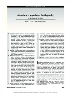
2.2 Electrical Properties of the Biological Tissues The electrical properties of the biological tissues are depend on the presence of body fluids. Moreover, those properties could be different for in vivo and in vitro analysis of the same tissue. The solid part of the tissue is mainly based on cellular membranes, which have the isolating properties. The presence of conductive fluid part and solid, isolating, component in the same tissue is affecting on anisotropic, electrical properties of the living tissue. Figure 2.1 (based on the results published by [67] presents the idealized curve of the changes in relative permittivity (er) of biological tissue with applied frequency. There are three major frequency ranges describing the changes of relative permittivity called the dispersion a, b and c. In some tissues not every range is clearly represented. Dispersion a, occurring in lower frequencies (around 100 Hz) is associated with interfacial polarization and ion transport across the cell membranes. The b-dispersion is related to the ‘‘capacitive shorting-out of membrane resistances, and rotational relaxations of biomacromolecules’’. The c-dispersion is origins from ‘‘the relaxation of bulk water in the tissue’’ [67]. The electrical properties of the tissues is analysed using impedance spectroscopy method. It allows to differentiate between the various tissues and the level of degeneration caused by the pathological processes, e.g. tumour development, ischemia and the process of rejection the transplanted organ [64, 95]. The mainstream researches on bioimpedance methods are presented regularly during the International Conferences on Electrical Bio-Impedance (ICEBI) organised worldwide every third year since the first meeting in 1969. The basic research achievements in that field was presented in the monograph written by Grimnes and Martinsen [28]. Fig. 2.1 An idealized curve of the changes in relative permittivity of biological tissue with applied frequency

2.2 Electrical Properties of the Biological Tissues Table 2.1

9

Type of the tissue

Resistivity (X cm)

Blood plasma Blood (for hematocrit Ht = 47%) Skeletal muscle (longitudinal) Skeletal muscle (transverse) Heart muscle (dog) Lungs (dog) Fat Saline 0.9%

63 150 300 700 750 1,200 2,180 57

In the impedance cardiography it is used the frequency range between 20 and 100 kHz. For that range the relative permittivity is at the level of several thousands (e.g. er = 5,000 for f = 50 kHz). The thin cellular membranes separating the conductive fluids create the electrical capacitances at the level up to 1 lF/cm2. This results in a resistive and capacitive character of the electrical properties of the biological tissues, with the absence of the symptoms of the inductive components. The lowest resistivity of biological material is observed in blood plasma (63 X cm). However considering the tissues blood has the lowest resistivity (150 X cm for Ht = 47%) and the highest one is observed for fat (1,275 X cm). The blood resistivity play a major role in the measurement of cardiac performance using impedance methods. It was assumed that the blood resistivity has an isotropic properties in static conditions, however there are some suggestions that flowing blood is characterized by a relative decreasing of resistivity by up to 10%. Moreover, some authors basing on experimental studies [96] and also model analysis claims that the anisotropic properties of flowing blood are much pronounced that we initially assumed and suggested to use the resistivity tensor. Table 2.1 presents the resistivity of different biological tissues and fluids basing on Geddes and Baker [23] compendium. The main conclusion drawn from the resistivity data presented in Table 2.1 is that in the impedance cardiography the change of the impedance signal is generated mainly by the changes caused by blood volume translocations. Other tissues are either not changing the volume or have at least 2 times higher resistivity. In the case of the heart muscle it is even 5 times higher, which leads to the conclusion that heart ‘‘isolates’’ the blood accumulated inside it.

2.3 Tissue as a Conductor The tissues could be treated as a finite, inhomogeneous volume conductor [44]. For the impedance cardiography applications we can also assume that it is a sourceless medium. The tissue impedance could be represented by three element model with

10

2 Impedance Cardiography

Fig. 2.2 The tissue impedance represented by three element model with single time constant

single time constant (Fig. 2.2). For this model it could be proposed the function, according to Cole–Cole model [13]. This function shows impedance Z as a function of frequency with real (R) and imaginary components (jX): Z(f) = R ? jX. In the expanded form it is presented below: Zðf Þ ¼ R1 þ

R 0  R1 R0  R1 R 0  R1 ¼ R1 þ  j-s 1 þ j-s 1 þ - 2 s2 1 þ - 2 s2

where Z(f) impedance as a function of frequency, R0 resistance at the frequency f = 0 Hz, R? resistance at the frequency f = ?, s time constant (RC2). The current passing through the biological tissues is described by the continuity condition divðr gradjÞ ¼ 0; where r, spatial conductivity of the tissue, u, electrical potential The Geselowitz theorem [26, 27] proposed the method of calculation the changes in impedance caused by the changes in volume, conductivity and movement of the organs in the body. Lehr [42] proposed the vector derivation method. Geselowitz work was more generalised by Mortarelli [56] considering modified geometry of the objects.

2.4 Frequency and Current Values There is general agreement to use the frequencies from the range 20-100 kHz and the sinusoidal current of the amplitude between 1 and 5 mA [92]. However some designers used a lower than suggested values of current. The lower boundary application is the suggestion leading to obtain the sufficient signal-to-noise ratio. The 1 mA current can create the muscle excitation at the lower than 20 kHz frequency. Also the skin–electrode impedance at 100 kHz is 100 times lower than in low frequencies. This helps to diminish the unwanted impact of the changes in the skin-electrode impedance, occurring during motion, into measured cardiological signal. However increasing the frequency of the application current above the 100 kHz causes the problem of stray capacitances.

2.5 Bioimpedance Measurement Methods

11

2.5 Bioimpedance Measurement Methods 2.5.1 Biopolar and Tetrapolar Method There are two main methods of the bioimpedance measurement: bipolar and tetrapolar. In the bipolar method there are two electrodes which play a role of application and receiving in one. Near the electrodes the current density is higher than in other parts of the tissue, which results in a non-uniform impact into the total impedance measurement. The total impedance signal is a superposition of two components: the skin–electrode impedance (modified by blood flow-induced movement) and the original signal (e.g. caused by the blood flow). In practice it is difficult to separate them. The scheme of the bipolar impedance measurement is presented in Fig. 2.3. In a four-electrode (tetrapolar) the application electrodes and receiving are separated. Figure 2.4 presents the scheme of the tetrapolar impedance measurement, typical way of obtaining the impedance cardiography signal. The constant amplitude current oscillates between the application electrodes (A) and the voltage changes are detected on the receiving electrodes (R). This voltage, due to the constant amplitude of current is proportional to the impedance of the tissue segment limited by the band electrodes. The voltage changes, are proportional to the impedance changes between receiving electrodes. The main advantage of that method over the bipolar is that the current density distribution is more uniform. Another one is that the disturbing role of the electrode impedances is minimized.

2.5.2 Alternating Constant-Current Source The measured impedance and its changes is in series with stray impedances of the electrodes and cables. Webster [92] estimates the stray capacitances at 15 pF which results in impedance as large as 100 k (at the frequency 100 kHz of the oscillating current. Since the measured value has the impedance smaller than 30–35 (and its Fig. 2.3 The scheme of the bipolar impedance measurement. The constant amplitude current oscillates between the application electrodes and the voltage changes are detected on the same electrodes A1 and A2

12

2 Impedance Cardiography

Fig. 2.4 The scheme of the tetrapolar (four-electrode) impedance measurement. The constant amplitude current oscillates between the application electrodes (A1–A2) and the voltage changes are detected on the receiving electrodes (R1–R2)

changes are about 100 times lower) so the internal impedance of the alternating current source should be sufficiently high. In some applications the constant amplitude oscillating current is supplied via transformer with a low-capacity.

2.5.3 Receiving Unit The voltage is sensed at the receiving electrodes. Assuming that their stray impedances are at the same level as the application electrodes (100 k at the frequency 100 kHz), the input impedance of the detecting amplifier should be sufficiently high. The instrumentation amplifiers offered by many suppliers could be used to design the first stage of the circuit that satisfy this requirements. Assuming the current amplitude i = 1 mA and the base impedance Z = 20–35 X, we can assume that the maximal value of the voltage amplitude at the level v = Zi (20–35 mV). The most important signal is stroke volume calculations is the change in the main impedance. The observed change of the impedance (DZ) has an amplitude of 100–400 mX, which results in 0.1–0.4 mV signal for the 1 mA current. Increasing the amplitude of the applied current to 5 mA we could bring the base impedance signal (Z) and the change of the impedance (DZ) to the level of 100–175 and 0.5–2 mV, respectively. However, increasing the current amplitude is possible in the stationary system but very much limited in battery powered applications like Holter-type instrumentation [97].

2.5.4 Demodulation Unit The useful, small biological signal of low frequency is hidden in the large signal of the high frequency (20–100 kHz). Thus any amplitude demodulator AM could be used to extract the voltage signal proportional to the changes in the in the impedance. Some designers uses the phase-sensitive detectors which are insensitive to the mains frequency. At the output of the demodulator occurs the signal

2.5 Bioimpedance Measurement Methods

13

proportional to the sum of Z and DZ signals. So another functional unit is essential to provide separated Z and DZ signals. The Z base impedance (denoted later by Z0) is proportional to the content of blood in the segment limited by the receiving electrodes, whereas DZ is used to estimate stroke volume, systolic time intervals and derivative signals.

2.5.5 Automatic Balance Systems Any impedance system is very sensitive to the motion artefacts. The changes in the skin–electrode impedances caused by the body movement may result in the changes larger then physiologically justified variations. This may caused the saturation of the amplifier which could last even for more than 10 s. In stationary solutions the operator could manually initiate the adjustment unit which allows the momentary resets the DZ to zero. In the ambulatory solutions this process should be performed automatically, just to avoid the long time loss of the signal. The automatic balance system which distinguish the physiologically induced changes from the unwanted variations (caused by e.g. motion artefacts) for stationary solutions was described by Shankar and Webster [76]. The comparator-based solution was applied in the ambulatory system [14].

2.6 Electrodes Types and Topography There are several types of the electrodes topography used in generating of the impedance cardiography signals. Historically, the first was a set of four band electrodes. However, then occurred some modification of that techniques.

2.6.1 Band Electrodes, Spot Electrodes and Mixed Spot/Band Electrodes When band electrodes are applied, two of them were placed around the neck separated by few centimetres and one over the suprasternal notch and the last one 10 cm lower. Spot electrodes are placed at the same level on the chest as the band electrodes same positions as band electrodes. Figure 2.5 presents the typical position of band electrodes connected to the main parts of each impedance cardiography system—generator and receiver (amplifier/detector). Please note the distance between inner-receiving electrodes L0. The ECG electrodes are not presented. Some systems use the same electrodes for detecting ECG and generating ICG signal. Several researchers use the mixed topology of the electrodes substituting band electrodes by the easy to use, however more noisy spot electrodes (Fig. 2.6).

14

2 Impedance Cardiography

Fig. 2.5 The typical position of band connected to the main parts of each impedance cardiography system—generator and receiver (amplifier/detector) according to the scheme proposed by Kubicek et al. [39]. Please note the distance between inner-receiving electrodes L0. The ECG electrodes are not presented

Fig. 2.6 The topography of the electrodes used in the PhysioFlow Enduro device

2.6.2 Other Solutions The BioZ (and derivative) systems producers, as well as Task Force Monitor and PhysioFlow suggested their own topography of the electrodes. They could be found on the web pages of the respective producers (http://www.sonosite. com/products/bioz-dx, http://www.cnsystems.at/product-line/task-force-monitor/ features). Below please find the figure adapted from the materials on PhysioFlow Enduro device published on their web page.

2.7 Signal Description and Analysis

15

2.7 Signal Description and Analysis 2.7.1 Impedance Cardiography Traces The typical impedance cardiography traces accompanied by the one lead of ECG are presented in Fig. 2.7. On the first channel ECG is shown, on the second the first derivative of the DZ signal which is denoted dz/dt. Calibrations for the respective signals are also presented. In practice only ECG and the first derivative signal (dz/dt) are used to calculate the hemodynamic parameters. Another data essential to make those evaluations is the value of the base impedance (Z0), which is usually not changing very fast. So in some applications Z0 was stored as a only one value for several cycles. Figure 2.8 shows the traces of electrical (ECG-top line) and mechanical activity of the heart (dz/dt—bottom line) recorded for the one cycle of the heart. There are some characteristic points (waves) defined and the method of determination for some important periods of the heart cycle presented. All of those symbols and time periods determination are described in the following sub-chapters.

2.7.2 Characteristic Points on Impedance Cardiography Curves Following the method of description the characteristic points and waves in ECG traces using letters (PQRST) researchers suggested the similar way for impedance signal (dz/dt). Lababidi et al. [41] associated the some notches in the ICG (dz/dt curve) with the events in mechanical action of cardiac muscle. They

Fig. 2.7 The typical impedance cardiography traces: the changes in the dz/dt (first derivative of the DZ) signal denoted as dz/dt (2nd channel), recorded simultaneously with one lead of ECG (1st channel). Please note the way of determination of PEP, ET (LVET) and (dz/dt)max, here marked as ‘‘amp’’ (adapted from [16])

16

2 Impedance Cardiography

Fig. 2.8 The traces showing electrical (ECG-top line) and mechanical activity of the heart (dz/dt-bottom line) recorded for the one cycle of the heart. Symbols denote some characteristic points on the ECG and impedance traces and the definition of periods occurring during heart cycle

suggested A, B, (dz/dt)max, (sometimes denoted as E), X, Y, O and Z. Although there are some trials in drawing the conclusions from the qualitative differences in the morphology of the ICG signal for various groups of cardiac patients (as for the ECG signal) they still remains in the stage of ‘‘attempts’’ and ICG is mainly used for quantitative estimation of cardiac parameters. Those ‘‘attempts’’ are mainly associated with the diagnosis of the valves malfunction. Below are listed and described the main waves and notches of ICG signal. A (atrial wave)

B

This wave is associated with the atrial contraction and its amplitude is correlated with the ejection fraction of the left atrium. The modification in time coupling between P-ECG and A-ICG is especially pronounced in patients with heart blocs [79]. A-wave is not observed when atrial fibrillation occurs [88]. This wave is associated with the opening of the aortic valve. It occurs on the ascending part of the ICG curve before (dz/dt)max. It is assumed that B wave occurs at the level of baseline for the ICG curve. There are some suggestions that its length is correlated with the isovolumetric contraction time. Denotes the beginning of the ejection time (left ventricular ejection time). The precise identification of a B point on the impedance cardiograph waveform is an important for accurate calculation of systolic time intervals, stroke volume, and cardiac output [45, 47, 49, 50]. Sometimes identifying the location of the B point is problematic because the characteristic upstroke that serves as a marker of this point is not always apparent [43]. To avoid this problem it was introduced a reliable method for B point identification, based on the consistent relationship between the R to B interval and the interval between the R-wave and the peak of the dZ/dt function (called by them as RZ) [43]. Thy suggested the function relating RB to RZ (RB = 1.233RZ -

2.7 Signal Description and Analysis

E

X

Y O

Z

17

0.0032RZ2 - 31.59) which accounts for 90–95% of the variance in the B point location across ages and gender and across baseline and stress conditions. As they claim, this relation affords a rapid approximation to B point measurement that, in noisy or degraded signals, is superior to visual B point identification and to a derivative-based estimate [43]. ((dz/dt)max): This point is placed on the top position of the curve reflecting the maximal speed of the change in the impedance. It is associated with the maximal velocity of the ejection measured by using ultrasound methods [33]. There is sometimes a collision between the meaning of the (dz/dt)max as a top point on the ICG curve and (dz/dt)max considered as a maximal amplitude of the ICG signal measured from the baseline to the top of the curve. Perhaps the top point should be denoted only by E letter. Some other authors call them Z wave or just dz/dtmax Corresponds to the closure of the aortic valve (and second heart sound—S2). Described as a minimal value of dz/dt signal, occurring after maximum E. In some patients it is not well pronounced (older people) or is placed on the same level as Y point showing the bimodal pattern of this wave. This might cause to the misleading automatic determination of the ejection time Corresponds to the closure of pulmonic valve This wave is associated with changing of the volume during the diastolic phase of the cycle and opening snap of the mitral valve. The high value of the O wave (similar to E) might be the symptom of the bicuspid valve malfunction or the heart inefficiency during heart acute ischemia [80] This wave describes a decreeing following the O wave. It is associated with a third heart sound—S3

2.7.3 Characteristic Periods in Impedance Cardiography Q-B

R-E (R-Z)

Time between the onset of the electrical contraction of the chambers and the opening of the aortic valve. It is described as pre-ejection period (PEP) which is a sum of electromechanical delay (EMD) and isovolumetric contraction (IVC) Time between the R point in ECG and the maximal value of the impedance signal. Seigel et al. [75] found the high correlation coefficient (r = 0.88) between R-E and the time from R-ECG to maximal value in the first derivative of the pressure signal (dp/dtmax)

18

Q-E

B-X

2 Impedance Cardiography

for the left ventricle. It might be treated as an index of the left chamber performance Time between the Q in ECG and the maximal value of the dz/ dt signal. It used in calculation of so called Heather index of cardiac contractility [29] Time between the opening and closing of the aortic valve described as left ventricular ejection time or shortly (ejection time)—LVET (ET)

The most frequently used are PEP and ET since they have the direct association with cardiac systole and were earlier analysed using the polyphysiographic methods [36, 78].

2.7.4 Hemodynamic Indices There are some indices which could be calculated solely using ICG and ECG traces and in the other group there are indices calculated using the above mentioned and other parameters like characterising mean arterial blood pressure (MAP) and body surface area (BSA). There were introduced and/or described by many researchers [39, 41, 68, 85, 94] SV

CO

STR TFC

Heather index

Stoke volume (SV) expressed in millilitres [ml] is the basic volumetric parameter characterising the amount of blood ejected from the left ventricle in one cycle Cardiac output (expressed in [l min-1] or [dm3 min-1]) is the volume of blood pumped by the heart during 1 min. It is a product result of SV and heart rate (HR). Of course it could be also calculated as a sum of all SV values occurring during 1 min period Systolic time ratio (PEP/ET), the ratio of the two basic systolic time intervals considered as an index of cardiac contractility Total fluid content is the index of the presence of fluid in the thorax region. Practically it is the inverse value of the basic impedance Z0 expressed in the units of 1/kX or [(kX)-1] The cardiac contractility index defined as a ratio of the maximal amplitude of dz/dt signal to the Q-E period (expressed in [X/s2]. So it means the rate of impedance changes to the time in which they are performed from the electrical onset to the peak mechanical action

The different producers provide some other indices using the mentioned above characteristic points and periods evaluated from the ICG curve. Other hemodynamic indices are created as a normalised of those from the basic group or an

2.7 Signal Description and Analysis

19

arithmetical combination of them and other hemodynamic parameters. The important normalisation factor is body surface area (BSA) expressed in [m2] units and calculated using the Dubois and Dubois [19] formula: BSA ¼ 0:007184  W 0:425  H 0:725 ; where W is weight supplied in [kg], H is height in [cm]. Stroke index (SI) Cardiac index (CI) Systemic vascular resistance (SVR)

Systemic vascular resistance index (SVRI) Velocity index (VI) and acceleration index (ACI)

Left cardiac work (LCW)

Left cardiac work index (LCWI) Stroke work index (SWI)

SV can be indexed to a patient’s body size by dividing by body surface area (BSA) CO indexed to a patient’s body size by dividing by body surface area (BSA) can be calculated if cardiac output (CO), mean arterial pressure (MAP), and central venous pressure (CVP). SVR = (MAP–CVP)/CO. Since CVP is close to 0, it could be simplified to MAP/CO. The units are [(dyne 9 s)/cm5] or [MPa s/m3]. Typical values of SVR: 900–1,200 dyn s/cm5 (90– 120 MPa s/m3). Some authors use name of total systemic resistance (TSR) is an SVR normalized by division of SVR by BSA There are two specific parameters introduced by producers of the BioZ impedance system. VI is the maximum rate of impedance change, and is representative of aortic blood velocity. ACI is the maximum rate of change of blood velocity and representative of aortic blood acceleration An indicator of the amount of work the left ventricle must perform to pump blood each minute. This index reflects myocardial oxygen consumption. It is the product of blood pressure and blood flow. LCW is determined with the following equation: LCW = (MAP–PAOP) 9 CO 9 0.0144, where PAOP is Pulmonary Artery Occluded Pressure, or wedge pressure. When Pulmonary Artery Catheter is not applied, a default value of 12 mm Hg can be used because of PAOP’s minimal effect on LCW determination. LCW is measured in Watts [W] or other units of work LCW can be indexed to a patient’s body size by substituting Cardiac Index for Cardiac Output to yield LCWI = (MAP–PAOP) 9 CI 9 0.0144 pressure times blood volume ejected in one beat normalised by body surface area (BSA)

20

Mean systolic ejection rate (MSER) Vascular rigidity (VR) Ejection phase contractility index (EPCI)

2 Impedance Cardiography

It is a volume of blood ejected during ejection time (divided by LVET) and normalised by body surface area (BSA) The ratio of pulse pressure per stroke volume index (SVI) It is defined as EPCI = (dz/dt).maxTFC. Sramek suggested that the aortic blood peak flow is a mirror image of ejection phase myocardial contractility. Thus the rate of cardiovascular impedance changes over time (dz/dt) is an image of the aortic blood flow

Thus, there are different types of the indices based on the ECG and ICG signals regarding cardiac timing, contractility and another group of the indices constructed basing an the ICG signals and blood pressure and/or body characterizing parameters. I am sure that researchers will develop some other indices showing their correlation with physiological variables or finding the new exponents of cardiac work, contractility or the efficiency of the heart pump.

2.7.5 The Influence of Breathing Breathing modulates the impedance signal causing its fluctuation around the base impedance Z0 which results in ‘‘moving baseline’’ of dz/dt signal. This might result in the misleading absolute value calculations of SV when the ‘‘stiff zero level’’ is used to find the maximal amplitude of the dz/dt trace. Thus the base line should be determined separately for each cycle or this modulating effect of breathing should be removed from the signal. Slow fluctuations of the ICG signal around the base line caused by breathing could be eliminated by using the following methods: 1. temporary elimination of breathing, used by Dennistone et al. [17], Keim et al. [31] and Du Quesnay et al. [18]; 2. application of an ensemble averaging method to provide the ‘‘mean cycle’’ for the certain period [48, 58]; 3. digital filtering [51, 91]. Du Quesnay et al. [18] noted that temporary elimination of breathing affects SV despite the reduction of breathing modulation. Moreover, it is not possible to perform some physiological tests when not breathing (e.g. exercise tests). Application of an ensemble averaging technique means that information regarding beatto-beat changes is lost. Thus filtering is the best method of reducing the interference of breathing modulation with the ICG signal.

2.7 Signal Description and Analysis

21

2.7.6 The Origin of the Impedance Cardiography Signals In impedance cardiography it is usual to use alternating current of frequency in the range of f = 20–150 kHz and with constant amplitude (range 0.5–5 mA), oscillating between application electrodes A1–A2 (Fig. 2.5) and meeting the impedance of a significant real component (15–30 X) and a negligible (causing a 10 phase shift) imaginary component. Blood is a tissue characterised by the highest conductivity. Its resistivity (130–160 X cm) is two times lower than the resistivity of muscle tissue (300 X cm), which is second on the list ranged from low to high values. Also, blood’s resistivity is many times higher than the resistivity of other tissues [23, 24]. This biophysical property of the blood means that the impedance between receiving electrodes is mainly caused by the volume of blood contained within this segment of the chest. Nyboer’s formula (explained below) was a mathematical description of a simple model of the changes in blood vessels in the chest during cardiac cycle. It presented the chest, as a uniform cylinder in which there was a single blood vessel of a particular diameter filled with blood. The blood ejection from heart to the aorta during contraction was simulated as a rapid extension of this vessel (uniform increase of diameter) and the similarly, rapid uniform return after closing the aortic valve. The time of the vessel extension was equal to the ejection time. This simplified model of the heart hemodynamics phenomena and its consequences when SV was calculated were many times criticised by both enthusiasts, [7] and Porter and Swain [69], and opponents of the ICG method, [30] and Keim et al. [31]. This criticism was an inspiration for studies where the impact of particular components into ICG signal was evaluated [2, 9, 34, 38, 65, 74, 77, 90]. The validity of one-cylinder model was questioned by [71], who suggested the serial connected two-cylinder model instead. They studied the length (distance between the receiving electrodes) dependence of the impedance parameters Z0, (dz/dt)max, and stroke volume (SV) in both models. It was shown that, within a one-cylinder model, all parameters are directly proportional to the length, whereas, if the volume conduction of the thorax and the neck are modelled separately, Z0 and (dZ/dt)min were expected to be linear dependent and SV was non-linear upon the length. Those expectations were compared to results from in vivo measurements [71] using an electrode arrays placed o the thorax. The results showed a nearly linear relation between the ICG parameters and the length except for small distances. Regression analysis of the linear part revealed statistically significant intercepts (p \ 0.05). When stroke volume was calculated using Kubicek’s equation, neither the intercept nor the non-linear part could be explained by a onecylinder model, whereas a model consisting of two cylinders serially connected described the experimental results accurately. Thus they concluded that SV estimation based on a one-cylinder model is biased due to the invalid one-cylinder model and suggested the corrections for the Kubicek equation using their twocylinder model [71].

22

2 Impedance Cardiography

It may be concluded that the following mechanical phenomena occurring during cardiac cycle and give impact to the impedance cardiography signal when the alternating current passes the chest: 1. 2. 3. 4.

the aorta’s and the neck artery’s extension caused by arterial pulse pressure, the pulmonary vessels’ extension, changes in the volume of heart and the volume of blood filling it, changes in the volume of blood filling the pulmonary vessels, resulting in an increase of the lungs’ conductivity, 5. changes in the blood resistivity in the large vessels caused by reorientation of the blood cells as a function of the velocity of blood flow, 6. changes in skeletal muscle resistivity caused by the pulse blood flow. Shankar et al. [77], Kosicki et al. [38] and Patterson [65], presented a mathematical model of the impedance changes in the chest that occur during the cardiac cycle. Kim et al. [34], based on the finite element model and analysing the impact of the factors described in points 1, 3, 4, 5. They concluded that changes in impedance are proportional to the extension of the aorta and that modification of the lung’s resistivity has an eight times’ smaller impact than that of the aorta. The impact of the heart signal on base impedance was significant but not proportional to changes in heart volume. These findings were confirmed by Kosicki et al. [38], who presented a cylindrical model of the chest with non-coaxial positioning of the chest organs. They noticed the small phase of the aortic signal in comparison to changes of resistivity during blood flow. They also presented the magnitude and phase shift of the particular components of the impedance signal. Patterson [65], however, on the basis of a three-dimensional resistors model concluded that the impact on the impedance signal of particular components is: the pulmonary component (61%), main arteries (23%), skeletal muscle (13%), and other sources (3%). Most of these papers were theoretical and checked only on ‘‘phantom’’ physical models. The problem of whether the impact of the aortic or the pulmonary artery is higher was solved by Thomsen [90], who experimentally found a higher correlation between impedance SV and aortic blood pressure (r = 0.63) than between SV and pulmonary artery blood pressure (r = 0.26). Additionally experiments performed by Bonjer et al. [9], on dogs (isolating the heart and lungs in a rubber bag) showed that heart muscle has a negligible impact to the ICG signal. There were several theoretical and experimental studies performed with the aim to determine the origin of the impedance signal. Penney [66], basing on several studies, summarised the contribution of the size and function of anatomical structures into the impedance cardiography signals. The result of this resume is presented in Table 2.2. Mohapatra [53] after the analysis of several hypotheses regarding the origin of the impedance cardiography signals concluded that the impedance changes were caused only by cardiac hemodynamics. He suggested that the signal reflects both a change in the blood velocity and change in blood volume. Moreover, the changing speed of ejection has its major effect on the systolic part of DZ whereas the

2.7 Signal Description and Analysis Table 2.2 Origin of the impedance signal in impedance cardiography (based on [66]

23

Contributing organ

Contribution (%)

Pulmonary artery and lungs Aorta and thoracic musculature Right ventricle Left ventricle Pulmonary vein and left atrium Vena cava and right atrium

+60 +60 -30 -30 +20 +20

changing volume (mainly of the atria and great veins) affects the diastolic portion of the impedance curve. Amidst the controversies regarding the unclear source of impedance cardiography signal, pointed out again by Mohapatra [54] and some other researchers, the correlation coefficients between the values obtained by ICG and reference methods has acceptable levels. On the basis of the results of these papers several conclusions could be drawn: 1. The ICG signal is complex and its components are not synchronised in phase and direction, 2. The proportions between its components are not well defined, 3. The ICG signal is dependent on the changes in the diameter of the aorta, neck arteries and pulmonary vessels and in the resistivity of flowing blood caused by blood cell reorientation (only in the large vessels), 4. The ICG signal appears not to be dependant on heart volume and the amount of blood in it (isolating properties of the heart muscle in relation to blood resistivity), 5. For typically positioned electrodes the ICG signal is not dependent on pulmonary artery extension.

2.7.7 The Methods of Stroke Volume Calculation There are different methods of calculation a stroke volume (and in the consequence other hemodynamic parameters) using impedance signal, the characteristic points on the impedance waveform and parameters describing the physical dimension of the analysed segment of the human body. The usage of the different formulas may lead to the marked scattering of the results. Historically, the first was Kubicek formula [39, 40] derived from the Nyboer works [62, 63] signal. Let me describe shortly some of the formulas and methods using the ‘‘historical’’ order. Nyboer Formula Atzler and Lehman [3], for the first time suggested that changes in electrical impedance of the chest are related to the blood volume translocation in the thorax observed during the cardiac cycle. Their investigations were developed by Nyboer

24

2 Impedance Cardiography

et al. [62] and Nyboer [63], who presented a formula describing the relationship between changes in blood volume in any segment of the body and the changes in its impedance: DV ¼ q  L20  Z02  DZ where DV, changes of the blood volume of the body segment [cm3]; q, blood resistivity [X cm]; L0, distance between receiving electrodes [cm]; Z0, basic impedance of the body segment limited by receiving electrodes [X]; DZ, changes of the impedance of the segment limited by receiving electrodes [X]. It is generally accepted that changes in the thoracic impedance DZ are caused mainly by the ejection of blood from the left chamber to the aorta and are proportionate to the stroke volume (SV). Kubicek et al. [39] suggested this interpretation in 1966.

Kubicek Formula Kubicek suggested modification of Nyboer’s formula (2.1) replacing DZ = (dz/ dt)maxET, and substituting DV = SV, in a cardiac version of the impedance method [39, 40]. This resulted in establishing the basic impedance cardiography formula named after Kubicek: SV ¼ q  L20  Z02  ðdz=dtÞmax ET where SV stroke volume [cm3], (dz/dt)max, the maximum of the first derivative of the impedance signal [X/s], ET, ejection time [s], time of blood ejection from the left chamber, determined by selection of characteristic points on (dz/dt) trace, (other symbols are explained with Nyboer formula above).

Sramek Formula Sramek proposed another method of calculating stroke volume using 3 components: volume of electrically participating tissues (VEPT—which is a function of patient’s gender, height and weight), ventricular ejection time (VET), which has the similar meaning as LVET or ET in Kubicek formula and the ejection phase contractility index (EPCI), which is a product of maximal amplitude of the dz/dt signal (dz/dt)max and TFC (which is an Z-1 0 ). His idea was to show in the formula that SV is directly proportional to the physical size of a patient (i.e., to VEPT—body habitus scaling constant), directly proportional to duration of delivery of blood into the aorta (i.e., to VET), and (SV is directly proportional to the peak aortic blood flow (i.e., to EPCI). This lead to the formula: SV = VEPT  VET  EPCI

2.7 Signal Description and Analysis

25

where VEPT, volume of electrically participating tissues (a function of patient’s gender, height and weight); VET, ventricular ejection; EPCI, ejection phase contractility index. When substituting the above symbols by the expression used in the Kubicek formula it gives: SV ¼

ð0:17HÞ3  ðdz=dtÞmax  ET 4:25  Z0

where H, the height of the subject in [cm], (dz/dt)max, is the maximal amplitude of the dz/dt signal [X/s], ET, left ventricular ejection time [s], Z0, the base impedance of the segment limited by the receiving electrodes [X]. Sometimes this formula is presented as: SV ¼

L30  ðdz=dtÞmax  ET 4:25  Z0

where L0, the distance between receiving electrodes [cm]; L0, is assumed to be 0.17 of the height of the subject. This resulted in occurrence of the factor 0.17H in the earlier formula.

Sramek-Bernstein Formula Some researchers use another formula for SV calculation called the SramekBernstein equation: SV ¼ d 

ð0:17HÞ3  ðdz=dtÞmax  ET 4:25  Z0

It is based on the assumption that the thorax is a truncated cone with length L and circumference C measured at the xiphoid level [4, 5, 84, 86]. It was checked that C/L ratio is equal to 3.0 regardless of age or sex (with the exception of newborns). Also L is assumed to be 0.17 of the height (H) and a correction factor (d) relating actual and ideal weight was introduced. Bernstein and Lemmens [6], suggested another formula called N (Bernstein). The formula is given below: sffiffiffiffiffiffiffiffiffiffiffiffiffiffiffiffiffiffiffiffiffi VITBV ðdz=dtÞmax SV ¼ 2   ET; Z0 n where VITBV, 16 W1.02 [ml], empirical formula for intra-thoracic blood volume estimation when W is expressed in [kg]. Dimensionless index of transthoracic aberrant conduction; the way of its determination is given in the mentioned paper [6]. They verified the results using N (Bernstein) with those obtained by thermodilution method in 106 cardiac postoperative patients and achieved the better

26

2 Impedance Cardiography

accordance between the measurements in comparison to the usage of the other formulas. The Kubicek, Sramek and Sramek-Bernstein equations are based on different methodological assumptions but both are able to provide a reliable SV estimation.

TaskForce Monitor Method The Kubicek formula is the consequence of the cylindrical model of the thorax applied in the theoretical considerations. Sramek noted that this model is too simple to give the precise determination of the SV. He abandoned the cylindrical model of thorax and assumed that the thorax is the frustum of a parameters dependant on some anthropometric parameters. Than introduced the volume of electrically participating tissues (VEPT), which is a function of patient’s gender, height and weight. The task force monitor, producers of stationary equipment, followed the way of the usage of anthropometric measures to estimate the electrically participating volume of the thorax named by them as (Vth) [22]. They noted that ‘‘shape of the body is neither an exact cylinder nor a frustum but more or less determined by the fact of whether the patient is underweight, normal or obese: underweight people will tend to have a more cylindrical thorax shape while obese people will have a more frustum-shaped thorax’’. Than they suggested that ‘‘the grade of leanness/obeseness can be estimated by the body mass index (BMI), whereby a BMI of 25 is considered to be the border between normal and marginal overweight’’ [22]. They used a tilt tests to determine the influence of the body composition as well as the base impedance Z0 on Vth. Thus the Vth is described according to the formula: Vth ¼ C1  H 3 

BMI n ; Z0m

where C1, powers m and n are subject to proprietary non-disclosure [22]. Since BMI is defined as W/H2, the following equation was implemented:  W n ðdz=dtÞmax  ET 2 3 SV ¼ C1  H  H m ; Z0 Z0 and after simplifications: SV ¼ C1 

W n  H 32n  ðdz=dtÞmax  ET Z0mþ1

PhysioFlow Method The PhysioFlow designers did not reveal the exact formula for SV calculations. The idea of that calculations were presented in the Appendix I of the paper by Charloux et al. [11].

2.7 Signal Description and Analysis

27

In contrary to the previous formulas they did not use the baseline values of the impedance Z0 or the physical parameter like a distance between the receiving electrodes L0, although they use BSA (so weight and height of the subjects). They used, however, the Haycock formula, BSA ¼ 0:024265 W 0:5378 H 0:3964 for BSA instead of that provided by Dubois and Dubois [19]. There are several steps in calculation of SV (or SVI) using PhysioFlow (they called SVI by SVi). Basing on the mentioned Appendix 1 from [11] let me describe those steps. A first evaluation of SVi, called SVical, is computed during a calibration procedure based on 24 consecutive heart beats recorded in the resting condition. The largest impedance variation during systole (Zmax–Zmin), and the largest rate of variation of the impedance signal (dZ/dt)max, called the contractility index (CTI) is stored. The SVi calculation depends on the ventricular ejection time (ET). The designers of the PhysioFlow have chosen to use a slightly different parameter, called the thoracic flow inversion time (TFIT), expressed in [ms]. The TFIT is the time interval between the first zero value following the beginning of the cardiac cycle (starting from QRS in ECG) and the first nadir after the peak of the ejection velocity (dZ/ d/max). Afterwards, the TFIT is weighted [W(TFIT)] using a specific algorithm where the pulse pressure (PP) (the difference between systolic arterial pressure and diastolic arterial pressure) and the momentary HR is used. They introduced their method of SV calculations basing on the assumptions that the aortic compliance contributes to the signal waveform. For example, Chemia et al. [12] have demonstrated the existence of a linear relationship between aortic compliance and the SV/PP ratio. In the algorithm the PP, calculated from a sphygmomanometer measurement, is introduced at the end of the Physio Flow calibration phase. Similarly, certain in relationship with. Second foundation of their method is the of the influence of the oscillatory and resonance phenomena on the ICG signal morphology. They spotted that Murgo et al. [57] described a relationship between the pressure waveform and aortic impedance or momentary HR. Thus they used the HR as a second factor entering into the algorithm. As a result of the above concepts, SVical is computed according to the following formula: SVical ¼ k ½ðdZ=dtmax Þ=ðZmax  Zmin ÞW ðTFITcal Þ where k is a constant, and the subscript ‘‘cal’’ indicates the parameters measured during the calibration phase. Thus SVical represents the baseline reference. During the data acquisition phase, the variations of the parameters described above are analysed and compared to those obtained during the calibration procedure. For instance, the designers demonstrated that the SV variations result mainly from a combination of contractility fluctuations (CTI) or (dz/dt)max changes and of TFIT variations. So, the stroke volume index is calculated basing on the calibrated value of SVi and the factor based on TFIC, CTI and their calibrated values:

28

2 Impedance Cardiography

SVi ¼ SVical ððCTI=CTIcal Þ : ðTFITcal =TFITÞÞ1=3 They claim that this concept is supported by a study by Moon et al. [55], who showed that changes in SV, for example during exercise, are correlated with variations in dz/dt, but inversely correlated with variations in left ventricular ejection time. They noted that in all equations used by other impedance cardiography devices, these two parameters appear as a product. The main advantage of that formula over other is that positioning of the electrodes is not critical, since Z0 evaluation is unnecessary.

2.7.8 Blood Resistivity Impact Since blood resistivity (q) is a proportional factor in SV calculations that use the Kubicek formula its unbiased determination is important for evaluation of SV. There are two approaches to this problem in the literature: assumption that r is constant and in the range of 130–150 X cm, [20, 40, 58, 69, 81], or determination of r as a second order or exponential function of hematocrit (Hct), [17, 24, 37, 89]. The supporters of the first approach have used resistivity closer to 130 X cm. Quail et al. used a transformed Kubicek formula to determine blood resistivity in dogs for different Hct and measured SV using a magnetic flowmeter [70]. For ±35% of Hct changes (range 0.22–0.66, mean 0.41) they observed only ±3.3% change in resistivity (range 141.3–132.2 X cm, mean 136.8 X cm). Moreover, the blood resistivity as a function of Hct was determined in vitro. However, Swanson and Webster estimated that blood resistivity is positively correlated with blood velocity and may change by 10% within the physiological range of the flow [87]. Thus it seemed that application of a constant value of r gives a smaller error than the introduction of another measurement (resistivity), which is out of control. Wtorek et al. also pointed out the anisotropy of the resistivity of flowing blood [95, 96]. The ICG method is sensitive to artefacts, so motion, anxiety, restlessness, shivering, and hyperventilation may interfere with measurements and modify physiologic responses. Factors preventing good electrode-to-skin contact (sweating, oils, and severe obesity) may also limit the accuracy of signal detection.

2.8 Signal Conditioning When it is not possible to eliminate the source of the noise the most important method for improving the signal to noise ration in impedance cardiography measurements is the averaging technique.

2.8 Signal Conditioning

29

2.8.1 Ensemble Averaging Method In impedance cardiography the ensemble averaging is a method for reduction of the influence of the artefacts or unwanted effect of other signals. It is used as a method of improvement a signal to noise ratio, when ‘‘noise’’ means not only the typical disturbances in signal detection (e.g. caused by motion) but also the signals modulating the original source of physiological changes. The crucial issue in that process is the method of synchronisation. When there is no other signal (like in ECG quality improvement) the gating is performed by the characteristic wave in the transformed signal (R-ECG). The respective wave in first derivative of the impedance signal (dz/ dt) would be the peak of it called dz/dtmax (some authors use dz/dtmin notation, just to mark that the direction of impedance changes is negative although usually presented as a positive). However, the peak value of dz/dt is also affected by shape modifications (including bimodality). Thus the signal averaging is usually synchronized by the signal of electrical activity of the heart—by R-ECG. It is performed over a certain period (e.g. 60 s) by summing the digitised samples gated by R-wave peak and dividing by the numbers of beats in the analysed period. Another approach of synchronizing by the peak value of the first derivative signal (dz/dt) was applied by Kim et al. [35]. They tested their method during four stages treadmill exercise. Stroke volumes of the five subjects averaged by the peak dz/dt were 0–23.5% higher than those obtained by the R point at rest and exercise. The ensemble averaging is used to reduce the influence of natural beat-to-beat variability and the disturbing effect of the respiration on impedance signal. The ensemble averaging was used in the stationary ICG by some authors [48, 58] and it is used also ambulatory version of ICG in VU-AMS [72]. This method may be used in on-line analysis or off-line calculations. Muzzi et al. [58] founded in stationary systems that ensemble-averaging of transthoracic impedance data provides waveforms from which ‘‘reliable estimates of cardiac output can be made during normal respiration in healthy human subjects at rest and exercise and in critically ill patients’’. Kelsey and Guethlein [32] compared cardiac parameters determined from ensemble averaged signals to those determined by simple beat-to-beat averaging over 60 and 20-s sampling intervals. They confirmed ‘‘validity of ensemble averaging as a method for deriving impedance cardiographic measures of myocardial performance’’. In one of the first research systems for portable ICG monitoring the signal averaging was performed on-line and the result was stored in the memory without the original trace, due to the memory size limitation [93]. The loss of the original signal was the main disadvantage of that method. Nowadays this restrictions disappeared due to the common availability of the memory cards in a variety of formats. Just to underline the tremendous progress in this area it is worth to mention that in 1993 the PCMCIA 20 MB Card produced by SanDisk (maximum capacity available on the market) cost about $1500. The cost of ultrafast compact flash card of 4 GB capacity in 2010 is below $50, and is decreasing. The largest capacity of 64 GB is sold at the price of below $350. Also the data transfer is very fast, currently at the rate of 20–30 MB/s. So the ensemble averaging method is used only to improve the signal to noise ratio

30

2 Impedance Cardiography

and extract the trends in long-term hemodynamic monitoring but not because of the memory capacity limitations.

2.8.2 Large-Scale Ensemble Averaging Method The large scale ensemble averaging method is a way of averaging longer than over the 60 s period. It was proposed by the group who developed the VU-AMS device [72]. This method was applied as a off-line analysis for a period of the similar type of the patient activity but lasting not longer than 1 h. If the activity type lasted longer than 1 h (sleeping) it was divided into several periods shorter than 1 h. The periods were selected using the entries from a patient diaries describing the activity, physical load, posture, location (home, work, etc.), and social situation. The full description of the categories is given by Riese et al. [72]. The morphology analysis of the large scale ensemble averaging was performed in a similar way to a 60 s averaging. The reason why the ensemble averaging method has been introduced was the demand of a precise, artefact free determination of Pre-ejection Period (PEP). PEP is a short systolic time interval beginning at Q-in QRS wave of ECG and ending at the moment of aortic opening derived from any signal showing the mechanical heart activity. The location of Q wave is not creating the significant error. But in case of ICG signal the ambiguous reading of the aortic valve opening might be a reason of substantial inaccuracy of PEP interval determination. When we assume roughly the range of PEP at the level 50–150 ms, the inaccuracy of 5 ms in the determination of that period creates a maximal error of 10% in one direction. However, 5 ms is not a maximal value of the inaccuracy in PEP determination. Ensemble averaging and/or large scale of the ensemble averaging are the methods leading to the PEP measurement improvement, minimizing the inaccuracy. Why accurate PEP measurement is so important? There are some suggestions that PEP absolute level correlates with sympathetic drive [10, 21]. Thus PEP would be an easy measure of sympathetic activity, useful in psychophysiological reactions to the stressors. Moreover, it was found that prolonged PEP occurs in patient with aortic stenosis [52]. Since PEP is strongly positively related to the level of venous return (pre-load) it could be also considered as a measure of it [82]. Also PEP expressed as a fraction of left ventricular ejection time (LVET) could be treated as a measure of cardiac contractility [1, 45].

2.9 Technical Aspects of ICG-Limitations, Errors and Patients’ Safety Evaluation of SV by ICG, like any indirect measurement method, is biased by the superposition of partial errors. Assuming that errors of determination of L0 and Z0

2.9 Technical Aspects of ICG-Limitations, Errors and Patients’ Safety

31

are 1%, for ET -1.7% (5 ms of the time resolution for 200 Hz sampling frequency), and for (dz/dt)max - 2% (resistivity is set constant) the minimal SV error could be estimated by a differential method to be at the level of about 4%. Swanson and Webster, noted that it is not possible to identify all sources of errors but gave technical requirements for instrumentation which limited the measurement error to 5% [87]. They suggested that the frequency of the application current should be within the range f = 20…150 kHz, the current amplitude i = 0.5…5 mA, the common mode rejection ratio of the input amplifier—CMRR [400, the input impedance—Rin [ 4 kX, the output impedance of the current generator Rout [ 20 kX, and the noise level Vn \ 0.5 lV. The range of current is limited by the acceptable level of noise and the current density (j B 5 mA cm-2). The frequency range is limited by the bioelectric properties of the tissues. Apart from errors due to indirect measurement and the technical limitations of the method other sources of errors are associated with the methodology employed—the simplified model of the chest, the disturbing influence of breathing and uncertainties in estimation of blood resistivity.

2.10 Modifications of ICG, and Other Impedance Techniques The specific modifications of the impedance technique are rheo-angiography and rheo-encephalography [64]. Another application of the impedance technique is an impedance multi-frequency spectroscopy used to characterise tissue [64]. Also some researchers are involved in development of electro-impedance tomography (EIT), including the electrical mammography [61].

2.11 Physiological and Clinical Applications of Impedance Cardiography The ICG method has been applied to evaluation of changes in cardiac output during exercise in many different studies, starting from those reported by Miyamoto et al. [48, 50, 51], Miles et al. [46]. Bogaard et al. [8] published a review of the possibilities of hemodynamic measurements by ICG during exercise. They concluded that, although ICG ‘‘derived stroke volume calculation is based on several debated assumptions, numerous validation studies have shown good accuracy and reproducibility, also during exercise’’. Moreover, [73], in their review stated that ‘‘impedance cardiography is becoming an accepted method for safe, reliable, and reproducible assessment of hemodynamics in heart failure’’. ICG has been successfully used in many studies performed in the author’s home laboratory on cardiovascular response to the handgrip [25], orthostatic manoeuvre [15] and other physiological tests including dynamic exercise [16, 98].

32

2 Impedance Cardiography

Also, the effects of 3 days of bed rest on hemodynamic responses to submaximal loads during graded exercise in athletes and men with sedentary lifestyles was analysed [83]. The controversies around the verification of ICG resulted in a sceptical approach by health authorities to this technique, which used to be considered a research and not clinical method. Thus Medicare and Medicaid Services and health insurance companies in USA used not to reimburse the cost of ICG usage [99]. This approach was changed (from 1 July 1999) and revised US policy on cardiac output monitoring by electrical impedance now allows limited coverage of cardiac monitoring using electrical bioimpedance, a form of plethysmography, for six uses: • • • • • •

Suspected cardiovascular disease Fluid management Differentiation of cardiogenic from pulmonary causes of acute dyspnoea Optimisation of pacemaker’s atrioventricular interval Determination of need for IV inotropic therapy Post-transplant myocardial biopsy patients

Insurance contractors may cover additional uses when they believe there is sufficient evidence of the medical effectiveness of such uses. Not covered is the use of such a device for any monitoring of patients with proven or suspected disease involving severe regurgitation of the aorta, or for patients with minute ventilation (MV) sensor function pacemakers, since the device may adversely affect the functioning of that type of pacemaker. Moreover these devices do not render accurate measurements in cardiac bypass patients when they are on a cardiopulmonary bypass machine though they do provide accurate measurements prior to and post bypass pump. Their detailed description may be found at http://new.cms.hhs.gov/manuals/downloads/Pub06_PART_50. pdf. Following the decision of Medicare and Mediaid Services in USA the respective national health institutions in other countries decided to allow refunding the impedance cardiography diagnosis, initially in a very limited areas, e.g. Intensive Care Units only. Certainly, these decisions are stimulating for the producers of the ICG equipment and hopefully will affect the development of the hemodynamic ambulatory monitoring systems based on impedance cardiography method.

2.12 Conclusions All of the ways of stroke volume calculation were verified using the clinically accepted reference techniques. Despite the methodological differences, real and assumed level of the error for this indirect measurement and the used model, it seems that the absolute values of the stroke volume plays a minor role in

2.12

Conclusions

33

ambulatory monitoring of the impedance signal. In that particular situation the patient is the reference for itself and the starting level of the SV is not so important when e.g. the hemodynamic effectives of the heart in arrhythmia events is visualised. In similar cases the percentage of the decrease in stroke volume could be give quantitative information on the acceptable level [59, 60]. In several clinical situations even a qualitative evaluation of the (dz/dt)max amplitude in neighbouring cycles (e.g. normal vs. trigeminy) would provide an additional diagnostic data.

References 1. Ahmed, S.S., Levinson, G.E., Schwartz, C.J., Ettinger, P.O.: Systolic time intervals as measures of the contractile state of the left ventricular myocardium in man. Circulation 46, 559–571 (1972) 2. Anderson Jr, F.A., Penney, B.C., Patwardhan, N.A., Wheeler, H.B.: Impedance plethysmography: the origin of electrical impedance changes measured in the human calf. Med. Biol. Eng. Comput. 18, 234–240 (1980) 3. Atzler, E., Lehmann, G.: Uber ein neues Verfahren sur Darstellung der Hertztatigkeit (Dielectrographi). Arbeitsphysiologie 5, 636–639 (1932) 4. Bernstein, D.P.: A new stroke volume equation for thoracic electrical bioimpedance: theory and rationale. Crit. Care Med. 14(10), 904–909 (1986) 5. Bernstein, D.P.: Continuous noninvasive real-time monitoring of stroke volume and cardiac output by thoracic electrical bioimpedance. Crit. Care Med. 14(10), 898–901 (1986) 6. Bernstein, D.P., Lemmens, H.J.: Stroke volume equation for impedance cardiography. Med. Biol. Eng. Comput. 43(4), 443–450 (2005) 7. Boer, P., Roos, J.C., Geyskes, G.G., Mees, E.J.D.: Measurement of cardiac output by impedance cardiography under various conditions. Am. J. Physiol. 237(4), H491–H492 (1979) 8. Bogaard, H.J., Woltjer, H.H., Postmus, P.E., de Vries, P.M.: Assessment of the haemodynamic response to exercise by means of electrical impedance cardiography: method, validation and clinical applications. Physiol. Meas. 18(2), 95–105 (1997) 9. Bonjer, F.H., van den Berg, J., Dirken, M.N.: The origin of the variations of body impedance occurring during the cardiac cycle. Circulation 6(3), 415–420 (1952) 10. Cacioppo, J.T., Uchino, B.N., Berntson, G.G.: Individual differences in the autonomic origins of heart rate reactivity: the psychometrics of respiratory sinus arrhythmia and preejection period. Pychophysiology 31(4), 412–419 (1994) 11. Charloux, A., Lonsdorfer-Wolf, E., Richard, R., Lampert, E., Oswald-Mammosser, M., Mettauer, B., Geny, B., Lonsdorfer, J.: A new impedance cardiograph device for the noninvasive evaluation of cardiac output at rest and during exercise: comparison with the ‘‘direct’’ Fick method. Eur. J. Appl. Physiol. 82(4), 313–320 (2000) 12. Chemia, D., Hebert, J.L., Coirault, C., Zamani, K., Suard, I., Colin, P., Lecarpentier, Y.: Total arterial compliance estimated by stroke volume-to-aortic pulse pressure ratio in humans. Am. J. Physiol. 274, H500–H505 (1998) 13. Cole, K.S., Cole, R.H.: Dispersion and absorption in dielectrics. I. Alternating current field. J. Chem. Phys. 1, 341–351 (1941) 14. Cybulski, G., Ksia˛z_ kiewicz, A., Łukasik, W., Niewiadomski, W., Pałko, T.: Ambulatory monitoring device for central hemodynamic and ECG signal recording on PCMCI flash memory cards, pp. 505–507. Computers in Cardiology, IEEE, New York, NY, USA (1995) 15. Cybulski, G.: Influence of age on the immediate cardiovascular response to the orthostatic manoeuvre. Eur. J. Appl. Physiol. 73, 563–572 (1996)

34

2 Impedance Cardiography

16. Cybulski, G.: Dynamic Impedance cardiography—the system and its applications. Pol. J. Med. Phys. Eng. 11(3), 127–209 (2005) 17. Dennistone, J.C., Maher, J.T., Reeves, J.T., Cruz, J.C., Cymerman, A., Grover, R.F.: Measurement of cardiac output by electrical impedance at rest and during exercise. J. Appl. Physiol. 30, 653–656 (1976) 18. Du Quesnay, M.C., Stoute, G.J., Hughson, R.L.: Cardiac output in exercise by impedance cardiography during breath holding and normal breathing. J. Appl. Physiol. 62(1), 101–107 (1987) 19. DuBois, D., DuBois, E.F.: A formula to estimate the approximate surface area if height and weight be known. Arch Intern. Med. 17, 863–871 (1916) 20. Ebert, T.J., Eckberg, D.L., Vetrovec, G.M., Cowley, M.J.: Impedance cardiograms reliably estimate beat-by-beat changes of left ventricular stroke volume in humans. Cardiovasc. Res. 18, 354–360 (1984) 21. Esler, M., Jennings, G., Lambert, G., Meredith, I., Horne, M., Eisenhofer, G.: Overflow of catecholamine neurotransmitters to the circulation: source, fate, and functions. Physiol. Rev. 70(4), 963–985 (1990) 22. Fortin, J., Habenbacher, W., Heller, A., Hacker, A., Grüllenberger, R., Innerhofer, J., Passath, H., Ch, Wagner, Haitchi, G., Flotzinger, D., Pacher, R., Wach, P.: Non-invasive beat-to-beat cardiac output monitoring by an improved method of transthoracic bioimpedance measurement. Comput. Biol. Med. 36(11), 1185–1203 (2006). (Epub 2005 Aug 29) 23. Geddes, L.A., Baker, L.E.: Specific resistance of biological material—a compendum of data for biomedical engineer and physiologist. Med. Biol. Eng. 5(3), 271–293 (1967) 24. Geddes, L.A., Sadler, C.: The specific resistance of blood at body temperature. Med. Biol. Eng. 5, 336–339 (1973) 25. Grucza, R., Kahn, J.F., Cybulski, G., Niewiadomski, W., Stupnicka, E., Nazar, K.: Cardiovascular and sympatho-adrenal responses to static handgrip performed with one and two hands. Eur. J. Appl. Physiol. Occup. Physiol. 59(3), 184–188 (1989) 26. Geselowitz, D.B.: On bioelectric potentials in an inhomogeneous volume conductor. Biophys. J. 7(1), 1–11 (1967) 27. Geselowitz, D.B.: An application of electrocardiographic lead theory to impedance plethysmography. IEEE Trans. Biomed. Eng. 18(1), 38–41 (1971) 28. Grimnes, S., Martinsen, Ø.: Bioimpedance and Bioelectricity Bbasics, 2nd edn. ElsevierAcademic Press, Amsterdam-London. ISBN:978-0-12-374004 (2008) 29. Heather, L.W.: A Comparison of Cardiac Output Values by the Impedance Cardiograph and Dye Dilution Techniques in Cardiac Patients. Progress Report no. Na 594500. National Aeronautics and Space Administration, Manned Spacecraft Center, Houston (1969) 30. Ito, H., Yamakoshi, K.I., Togawa, T.: Transthoracic admittance plethysmograph for measuring cardiac output. J. Appl. Physiol. 40(3), 451–454 (1976) 31. Keim, H.J., Wallace, J.M., Thurston, H., Case, D.B., Drayer, J.I., Laragh, J.H.: Impedance cardiography for determination of stroke index. J. Appl. Physiol. 41(5 Pt. 1), 797–799 (1976) 32. Kelsey, R.M., Guethlein, W.: An evaluation of the ensemble averaged impedance cardiogram. Psychophysiology 27(1), 24–33 (1990) 33. Kerkkamp, H.J.J., Heethaar, R.M.: A comparison of bioimpedance and echocardiography in measuring systolic heart function in cardiac patients. Ann. N Y. Acad. Sci. (Issue: Electrical Bioimpedance Methods: Applications to Medicine And Biotechnology) 873, 149–154 (1999) 34. Kim, D.W., Baker, L.E., Pearce, J.A., Kim, W.K.: Origins of the impedance change in impedance cardiography by a three-dimensional finite element model. IEEE Trans. Biomed. Eng. 12, 993–1000 (1988) 35. Kim, D.W., Song, C.G., Lee, M.H.: A new ensemble averaging technique in impedance cardiography for estimation of stroke volume during treadmill exercise. Front. Med. Biol. Eng. 4(3), 179–188 (1992) 36. Kizakevich, P.N., Teague, S.M., Nissman, D.B., Jochem, W.J., Niclou, R., Sharma, M.K.: Comparative measures of systolic ejection during treadmill exercise by impedance cardiography and Doppler echocardiography. Biol. Psychol. 36(1–2), 51–61 (1993)

References

35

37. Kobayashi, Y., Andoh, Y., Fujinami, T., Nakayama, K., Takada, K., Takeuchi, T., Okamoto, M.: Impedance cardiography for estimating cardiac output during submaximal and maximal work. J. Appl. Physiol. 45(3), 459–462 (1978) 38. Kosicki, J., Chen, L., Hobbie, R., Patterson, R., Ackerman, E.: Contributions to the impedance cardiogram waveform. Ann. Biomed. Eng. 14, 67–80 (1986) 39. Kubicek, W.G., Karnegis, J.N., Patterson, R.P., Witsoe, D.A., Mattson, R.H.: Development and evaluation of an impedance cardiac output system. Aerosp. Med. 37(12), 1208–1212 (1966) 40. Kubicek, W.G., Patterson, R.P., Witsoe, D.A.: Impedance cardiography as a non-invasive method for monitoring cardiac function and other parameters of the cardiovascular system. Ann. N. Y. Acad. Sci. 170, 724–732 (1970) 41. Lababidi, Z., Ehmke, D.A., Durnin, R.E., Leaverston, P.E., Lauer, R.M.: The first derivative thoracic impedance cardiogram. Circulation 41(4), 651–658 (1970) 42. Lehr, J.: A vector derivation useful in impedance plethysmographic field calculation. IEEE Trans. Biomed. Eng. 19, 156–157 (1972) 43. Lozano, D.L., Norman, G., Knox, D., Wood, B.L., Miller, B.D., Emery, C.F., Berntson, G.G.: Where to B in dZ/dt. Psychophysiology. 44(1), 113–119 (2007) 44. Malmivuo, J., Plonsey, R.: Bioelectromagnetism. Principles and Applications of Bioelectric and Biomagnetic Fields. Oxford University Press, Oxford (1995) 45. Meijer, J.H., Boesveldt, S., Elbertse, E., Berendse, H.W.: Method to measure autonomic control of cardiac function using time interval parameters from impedance cardiography. Physiol. Meas. 29(6), S383–S391 (2008) 46. Miles, D.S., Sawka, M.N., Hanpeter, D.E., Foster-Jr, J.E., Doerr, B.M., Frey, M.A.B.: Central hemodynamics during progressive upper- and lower-body exercise and recovery. J. Appl. Physiol. 57(2), 366–370 (1984) 47. Milsom, I., Sivertsson, R., Biber, B., Olsson, T.: Measurement of stroke volume with impedance cardiography. Clin. Physiol. 2, 409–417 (1982) 48. Miyamoto, Y., Takahashi, M., Tamura, T., Nakamura, T., Hiura, T., Mikami, T.: Continous determination of cardiac output during exercise by the use of impedance plethysmography. Med. Biol. Eng. Comput. 19, 638–644 (1981) 49. Miyamoto, Y., Tamura, T., Mikami, T.: Automatic determination of cardiac output using an impedance plethysmography. Biotelem. Patient Monit. 8, 189–203 (1981) 50. Miyamoto, Y., Hiuguchi, J., Abe, Y., Hiura, T., Nakazono, Y., Mikami, T.: Dynamics of cardiac output and systolic time intervals in supine and upright exercise. J. Appl. Physiol. 55(6), 1674–1681 (1983) 51. Miyamoto, Y., Hiura, T., Tamura, T., Nakamura, T., Hiuguchi, J., Mikami, T.: Dynamics of cardiac, respiratory, and metabolic function in men in response to step work load. J. Appl. Physiol. 52(5), 1198–1208 (1982) 52. Moene, R.J., Mook, G.A., Kruizinga, K., Bergstra, A., Bossina, K.K.: Value of systolic time intervals in assessing severity of congenital aortic stenosis in children. Br Heart J 37, 1113– 1122 (1975) 53. Mohapatra, S.N.: Noninvasive Cardiovascular Monitoring of Electrical Impedance Technique. Pitman, London (1981) 54. Mohapatra, S.N.: Impedance cardiography. In: Webster, J.G. (ed.) Encyclopedia of Medical Devices and Instruments, pp. 1622–1632. Wiley, New York (1988) 55. Moon, J.K., Coggan, A.R., Hopper, M.K., Baker, L.E., Coyle, E.F.: Stroke volume measurement during supine and upright cycle exercise by impedance cardiography. Ann. Biomed. Eng. 22, 514–523 (1994) 56. Mortarelli, J.R.: A generalisation of the Geselowitz relationship useful in impedance plethysmographic field calculation. IEEE Trans. Biomed. Eng. 27, 665–667 (1980) 57. Murgo, J.P., Westerhof, N., Giolma, J.P., Altobelli, S.A.: Aortic input impedance in normal man: relationship to pressure wave forms. Circulation 62(1), 105–116 (1980) 58. Muzzi, M., Jeutter, D.C., Smith, J.J.: Computer-automated impedance-derived cardiac indexes. IEEE Trans. Biomed. Eng. 33(1), 42–47 (1986)

36

2 Impedance Cardiography

59. Nakagawara, M., Yamakoshi, K.: A portable instrument for non-invasive monitoring of beatby-beat cardiovascular haemodynamic parameters based on the volume-compensation and electrical-admittance method. Med. Biol. Eng. Comput. 38(1), 17–25 (2000) 60. Nakonezny, P.A., Kowalewski, R.B., Ernst, J.M., Hawkley, L.C., Lozano, D.L., Litvack, D.A., Berntson, G.G., Sollers 3rd, J.J., Kizakevich, P., Cacioppo, J.T., Lovallo, W.R.: New ambulatory impedance cardiograph validated against the Minnesota Impedance Cardiograph. Psychophysiology 38(3), 465–473 (2001) 61. Nowakowski, A., Wtorek, J., Stelter, J.: Technical University of Gdansk Electroimpedance mammograph. IX International Conference on Bio-Impedance, Heidelberg, pp. 434–437 (1995) 62. Nyboer, J., Bango, S., Barnett, A., et al.: Radiocardiograms. J. Clin. Invest. 19, 773–778 (1940) 63. Nyboer, J.: Plethysmography. Impedance. In: Glasser, O. (ed.) Medical Physics, vol. 2, pp. 736–743, Year Book Publishers, Chicago (1950) 64. Pałko, T., Galwas, B.: Electrical properties of biological tissues, their measurements and biomedical applications. Automedica 17, 343–365 (1999) 65. Patterson, R.P.: Sources of the thoracic cardiogenic electrical impedance signal as determined by a model. Med. Biol. Eng. Comput. 23, 411–417 (1985) 66. Penney, B.C.: Theory and cardiac applications of electrical impedance measurements. CRC Crit. Rev. Bioeng. 13, 227–281 (1986) 67. Pethig, R.: Dielectric properties of body tissues. Clin. Phys. Physiol. Meas. 8(suppl. A), 5–12 (1987) 68. Pickett, B.R., Buell, J.C.: Usefulness of the impedance cardiogram to reflect left ventricular diastolic function. Am. J. Cardiol. 71(12), 1099–1103 (1993) 69. Porter, J.M., Swain, I.D.: Measurement of cardiac output by electrical impedance plethysmography. J. Biomed. Eng. 9(3), 222–231 (1987) 70. Quail, A.W., Traugott, F.M.: Effects of changing haematocrit, ventricular rate and myocardial inotropy on the accuracy of impedance cardiography. Clin. Exp. Pharmacol. Physiol. 8(4), 335–343, (1981) 71. Raaijmakers, E., Faes, J.C., Goovaerts, H.G., de Vries, P.M.J.M., Heethaar, R.M.: The inacuracy of Kubicek’s one-cylinder model in thoracic impedance cardiography. IEEE Trans. Biomed. Eng. 44(1), 70–76 (1997) 72. Riese, H., Groot, P.F., van den Berg, M., Kupper, N.H., Magnee, E.H., Rohaan, E.J., Vrijkotte, T.G., Willemsen, G., de Geus, E.J.: Large-scale ensemble averaging of ambulatory impedance cardiograms. Behav. Res. Methods Instrum. Comput. 35(3), 467–477 (2003) 73. Rosenberg, P., Yancy, C.W.: Noninvasive assessment of hemodynamics: an emphasis on bioimpedance cardiography. Curr. Opin. Cardiol. 15(3), 151–155 (2000) 74. Sakamoto, K., Muto, K., Kanai, H., Iiuzuka, M.: Problems of impedance cardiography. Med. Eng. Comput. 17, 697–709 (1979) 75. Seigel, J.H., Fabian, M., Lankau, C., Levine, M., Cole, A., Nahmad, M.: Clinical and experimental use of thoracic impedance plethysmography in quantifying myocardial contractility. Surgery 67, 907–917 (1970) 76. Shankar, T.M.R., Webster, J.G.: Automatically balancing electrical impedance plethysmography. J. Clin. Eng. 9, 129–134 (1984) 77. Shankar, T.M.R., Webster, J.G., Shao, S.-Y.: The contribution of vessel volume change to the electrical impedance pulse. IEEE Trans. Biomed. Eng 1, 42–47 (1986) 78. Sherwood, A., McFetridge, J., Hutcheson, J.S.: Ambulatory impedance cardiography: a feasibility study. J. Appl. Physiol. 85(6), 2365–2369 (1998) 79. Siebert, J.: Impedance cardiography—atrio-ventricular heart blocs (in Polish). Elektrofizjologia i Elektrostymulacja Serca 2, 28–34 (1995) 80. Siebert, J., Wtorek, J.: Impedance cardiography. The early diastolic phase of heart chambers feeling—O dz/dt. (in Polish). Ann Acad Gedan 23, 79–89 (1993) 81. Smith, J.J., Bush, J.E., Wiedmeier, V.T., Tristani, F.E.: Application of impedance cardiography to study of postural stress. J. Appl. Physiol. 29(1), 133–137 (1970)

References

37

82. Smith, J.J., Muzi, M., Barney, J.A., Ceschinn, J., Hayes, J., Ebert, T.J.: Impedance-derived cardiac indices in supine and upright exercise. Ann. Biomed. Eng. 17(5), 507–515 (1989) 83. Smorawin´ski, J., Nazar, K., Kaciuba-Uscilko, H., Kamin´ska, E., Cybulski, G., Kodrzycka, A., Bicz, B., Greenleaf, J.E.: Effects of 3-day bed rest on physiological responses to graded exercise in athletes and sedentary men. J. Appl. Physiol. 91, 249–257 (2001) 84. Sramek, B.B.: Cardiac output by electrical impedance. Med. Electron. 13(2), 93–97 (1982) 85. Sramek, B.B.: Hemodynamic and pump-performance monitoring by electrical bioimpedance: new concepts. Probl. Resp Care 2(2), 274–290 (1989) 86. Sramek, B.B.: Thoracic electrical bioimpedance: Basic principles and physiologic relationship. Noninvas Cardiol 3(2), 83–88 (1994) 87. Swanson, D.K., Webster, J.G.: Errors in four-electrode impedance plethysmography. Med. Biol. Eng. Comput. 21(6), 674–680 (1983) 88. Takada, K., Fujinami, T., Senda, K., Nakayama, K., Nakano, S.: Clinical study of ‘‘A waves’’ (atrial waves) in impedance cardiograms. Am. Heart J. 94(6), 710–717 (1977) 89. Tanaka, K., Kanai, H., Nakayama, K., Ono, N.: The impedance of blood: the effects of red cell orientation and its application. Jpn. J. Med. Eng. 8, 436–443 (1970) 90. Thomsen, A.: Impedance cardiography—Is the output from right or from left ventricle measured ? Intensive Care Med. 6, 206 (1979) 91. Yamamoto, Y., Mokushi, K., Tamura, S., Mutoh, Y., Miyashita, M., Hamamoto, H.: Design and implementation of a digital filter for beat-by-beat impedance cardiography. IEEE Trans. Biomed. Eng. 12, 1086–1090 (1988) 92. Webster, J.G. (ed.): Medical Instrumentation. Application and Design. Wiley, New York (2010) 93. Willemsen, G.H., De Geus, E.J., Klaver, C.H., Van Doornen, L.J., Carroll, D.: Ambulatory monitoring of the impedance cardiogram. Psychophysiology 33(2), 184–193 (1996) 94. Winter, U.J., Klocke, R.K., Kubicek, W.G., Niederlag, W. (eds): Thoracic Impedance Measurements in Clinical Cardiology. Thieme Medical Publishers, New York (1994) 95. Wtorek, J., Polin´ski, A., Stelter, J., Nowakowski, A.: Cell for Measurements of Biological Tissue Complex Conductivity, Technology and Health Care, vol. 6, pp. 177–193. IOS Press (1998) 96. Wtorek, J., Polin´ski, A.: The contribution of blood-flow-induced conductivity changes to measured impedance. IEEE Trans. Biomed. Eng. 52(1), 41–49 (2005) 97. Zhang, Y., Qu, M., Webster, J.G., Tompkins, W.J.: Impedance cardiography for ambulatory subjects. In: Proceedings of the Seventh Annual Conference of the IEEE/Engineering in Medicine and Biology Society. Frontiers of Engineering and Computing in Health Care, vol. 2, pp. 764–769. IEEE, New York (1985) 98. Ziemba, A.W., Chwalbin´ska-Moneta, J., Kaciuba-Uscilko, H., Kruk, B., Krzeminski, K., Cybulski, G., Nazar, K.: Early effects of short-term aerobic training. Physiological responses to graded exercise. J. Sports Med. Phys. Fitness 43(1), 57–63 (2003) 99. Web page of Medicare and MediAid: http://new.cms.hhs.gov/manuals/downloads/Pub06_ PART_50.pdf

http://www.springer.com/978-3-642-11986-6