Chapter 2

Fundamental Concepts of Compositional Data Analysis

Abstract Compositional data is considered a statistical scale in its own right, with its own natural geometry and its own vector space structure. Compositional data analysis and this book cannot be understood without a basic knowledge of these issues and how they are represented in R. Therefore, this chapter introduces the basic geometric concepts of compositional data and of the R-package “compositions”: the relative nature of compositional data; how to load, represent, and display compositional data in R; the various compositional scales and geometries and how to select the right geometry for the problem at hand; and how to specify the geometry in “compositions” using the basic classes “acomp”, “rcomp”, “aplus”, “rplus”, “ccomp”, and “rplus”. A concise guide to the most important geometry for compositional data, the Aitchison geometry, is also included. The whole book relies on these basic principles, and the reader should make him or herself familiar with them in Sects. 2.1–2.5 before going on.

2.1 A Practical View to Compositional Concepts 2.1.1 Definition of Compositional Data A composition is often defined as a vector of D positive components x D Œx1 ; : : : ; xD  summing up to a given constant , set typically equal to 1 (portions), 100 (percentages), or 106 (ppm). We already mentioned that this definition is misleading, because many compositional datasets do not apparently satisfy it. Let us see how. Consider, for instance, this simple example of compositional data collected from typical nutrition tables of foodstuff in any kitchen cupboard: soy peas

Fat 7 3

Sodium 14 12

Carbonates Protein 10 13 61 22

Total 100 100

K.G. van den Boogaart and R. Tolosana-Delgado, Analyzing Compositional Data with R, Use R!, DOI 10.1007/978-3-642-36809-7 2, © Springer-Verlag Berlin Heidelberg 2013

13

14

2 Fundamental Concepts of Compositional Data Analysis

wheat corn beans

1 1 0.5

15 180 680

60 15 30

23 2 12

100 82 NA

This data can be loaded from a text file1 into R with the command read.table: > library(compositions) > kitchen (coi amounts amounts soy peas wheat corn beans

Fat Carbonates Protein 7.0 10 13 3.0 61 22 1.0 60 23 1.0 15 2 0.5 30 12

and then compute the total grams of each column by > (sumPresent Other Amounts clo(Amounts) soy peas wheat corn beans

Fat Carbonates Protein Other 0.07000 0.1000 0.13000 0.7000 0.03000 0.6100 0.22000 0.1400 0.01000 0.6000 0.23000 0.1600 0.01220 0.1829 0.02439 0.7805 0.01176 0.7059 0.28235 NA

The cbind command (for column bind) binds the columns of its arguments to a joint dataset containing all the columns. Of course, this procedure is only applicable when we know how much sample was analyzed in order to subtract from it the sum of the present components. This completion procedure has an advantage over the reclosure of the observed subcomposition: the reclosure loses all information about how much we had in total of the observed components, whereas in the completion procedure this total present is inherited by the “Other” part. A look at the last line reveals a practical problem of both the closure and the completion procedures in the presence of missing values. To close a composition with missing elements, we need to guess a value for the missing elements. The computer cannot add up unknown values and thus will close the rest of the

3

The different compositional classes will be discussed in Sect. 2.4.

2.1 A Practical View to Compositional Concepts

17

composition to 1, such as if this last components would be absent. However, it is very unlikely that the canned beans do not contain a considerable amount of water.

2.1.4 Compositions as Equivalence Classes Either by reclosing a subcomposition or by completing the composition, the dataset is now compositional in nature, since its columns sum up to a constant. In any way, we homogenized the totals to the same quantity, that is to say: we removed the information on the total amount of each sample. This is licit, because that total is in our kitchen example not relevant to evaluate the nutritive character of the different crops: it is an arbitrary choice of the producer or due to the local unit system. In fact, we could rescale each row of the dataset by multiplying it with a positive value, and the information they convey would not change. We can thus say that two vectors are compositionally equivalent (Aitchison, 1997; Barcel´o-Vidal, 2000) if one is simply some multiple of the other: a DA b , exists s > 0 for all i W ai D sbi In other words, all vectors with positive entries that are scaled versions of one another represent the same composition. For instance, the following three vectors are the same composition > Amounts[4,]*100/82 Fat Carbonates Protein Other corn 1.22 18.29 2.439 78.05 > Amounts[4,] corn

Fat Carbonates Protein Other 1 15 2 64

> acomp(Amounts[4,]) Fat Carbonates Protein Other corn 0.0122 0.1829 0.02439 0.7805 attr(,"class") [1] acomp first giving the composition of corn as portions of 100 g or mass %, then as portions of 82 g, and finally, as relative portions of 1. Note that in the last case, we used the command acomp, which tells the system to consider its argument as a compositional dataset, implicitly forcing a closure to 1. The different compositional classes (like acomp, or rplus before) are the grounding blocks of “compositions” and will be discussed in detail in Sect. 2.4.

18

2 Fundamental Concepts of Compositional Data Analysis

2.1.5 Perturbation as a Change of Units Indeed mass percentage is a quite irrelevant type of quantification for us: we are more interested in the energy intake. But the different nutrients have a different energy content (in kJ/g): > (epm (ec fatDataset total.Fat soy 7 peas 3 wheat 1 corn 1 beans 0.5

sat.Fat 1.40 0.60 0.25 0.32 0.10

unsat.Fat 5.60 2.40 0.75 0.68 0.10

we amalgamated them into the total fats. Amalgamation, though very commonly done, is a quite dangerous manipulation: a fair amount of information is lost in a way that we may find ourselves unable to further work with the amalgamated dataset. For instance, if saturated and unsaturated fats have different energy content, we cannot compute the total fat mass proportion from the total fat mass energy content, or vice-versa. Amalgamation thus should only be applied in the “definition of the problem” stage, when choosing which variables will be considered and in which units. It should be meaningful in the units we are dealing with, because afterwards, we will not be able to change them. And it should have a deep connection with our questions: to amalgamate apples and pears may be meaningful when investigating the nutrition habits of one population (where an apple may be equivalent to a pear) and catastrophic when studying the importance of some fruits in several cultures (where we just want to see different patterns of preference of fruits). Once the parts are defined, the units chosen, and the questions posed, we should not amalgamate a variable anymore. The easiest way to amalgamate data in R is to explicitly compute the amalgamated components as totals of an unclosed amount dataset (of an amount class, "rplus" or " aplus") containing only these components: > fatDataset$total.Fat = totals(aplus(fatDataset, c("sat.Fat","unsat.Fat")))#$ The aplus command works in the same way as acomp but explicitly states that the total is still relevant and no reclosure should be performed. It is used to assign the scale of a dataset of amounts in relative geometry. Amalgamation is further explained in Sect. 3.3.1.

20

2 Fundamental Concepts of Compositional Data Analysis

2.1.7 Missing Values and Outliers Note that the total amount for beans is missing (the nutrition table was reported for a 250 mL can of this product). We could have more missing values in the dataset by considering potassium, which is only given for some of the products, probably those for which it is relevant. However, it would be naive to assume that there is no potassium in any of these products. Much more than in classical multivariate analysis, missing values in compositional data need a careful treatment, especially because a missing value in a single component makes it impossible to close or complete the data, such that finally, the actual portion of no single component is known. It will be thus very important to understand which procedures are still valid in the presence of missing values and how others might be (partially) mended. The same applies to many other kinds of irregularities in compositional data, like measurements with errors, atypical values, or values below the detection limit: in all these cases, the total sum will either be unknown or affected by an error, which will propagate to all the variables by the closure. The solution comes by realizing that whichever this total value might be, the (log)ratios between any regular components are unaffected. The “compositions” package will thus close the non-missing parts as if the missing parts are 0, knowing that this value will not affect any proper analysis.

2.2 Principles of Compositional Analysis Any objective statistical methodology should give equivalent results, when applied to two datasets which only differ by irrelevant details. The following four sections present four manipulations that should be irrelevant for compositions and that thus generate four invariance principles, with far-ranging consequences for the mathematics underpinning compositional data analysis (Aitchison, 1986).

2.2.1 Scaling Invariance For the theoretical approach taken in this book, we will consider a vector as a composition whenever its components represent the relative weight or importance of a set of parts forming a whole. In this case, the size or total weight of that whole is irrelevant. One can then remove that apparent influence by forcing the data vectors to share the same total sum  with the closure operation, C .x/ D

x : 1t  x

(2.1)

The components xi of a closed composition x D .x1 ; x2 ; : : : ; xD / are values in the interval .0; 1/ and will be referred to as portions throughout this book. The term proportions will be reserved for ratios and relative sizes of components.

2.2 Principles of Compositional Analysis

21

By applying the closure, we can compare data from samples of different sizes, e.g., the beans, corn, and wheat in our simple kitchen example (even though their compositions were respectively reported for 100 g, 82 g, and 250 mL of product); a sand/silt/clay composition of two sediment samples of 100 g and 500 g; and the proportion of votes to three parties in two electoral districts of 106 and 107 inhabitants. For instance, the vectors a D Œ12; 3; 4, b D Œ2400; 600; 800, c D Œ12=17; 3=17; 4=17, and d D Œ12=13; 3=13; 4=13 represent all the same composition, as the relative importance (the ratios) between their components is the same. A sensible compositional analysis should therefore provide the same answer independently of the value of  or even independently of whether the closure was applied or else the data vectors sum up to different values. We say the analysis will be then scaling invariant. Aitchison (1986) already showed that all scaling-invariant functions of a composition can be expressed as functions of log ratios ln.xi =xj /.

2.2.2 Perturbation Invariance Compositional data can be presented in many different units, and even when given in portions, it is still relevant in which physical quantities the components were originally measured: g, tons, mass %, cm3 , vol. %, mols, molalities, ppm, ppb, partial pressure, energy, electric loading, money, time, persons, events, cells, mineral grains, etc. Even if it is clearly defined what substance we are measuring, how it is quantified is still a choice of the experimenter. It is extremely rare to find a composition where only one single type of quantification is meaningful: in most of the cases, several units could be equally chosen. And since different components are typically also qualitatively different, they might have different interesting properties. For instance, to change a mass proportion to a volume percentage, we need the densities of all components, which will be typically different. The same applies to changing prices between different valuations (from market price to book value, or to buying price, etc.), passing nutrition masses to energy intake, or cell type to energy consumption or biomass production. Thus, different analysts would end up having different values representing exactly the same compositions just due to a different choice of units. It is evident that the statistical analyses we can apply should thus give the same qualitative results regardless of the units chosen, as long as they contain the same information, i.e., as long as we can transform the units into each other, e.g., by rescaling each component by its density. This operation is done by a perturbation with a composition containing as entries the conversion factors (e.g., the densities) for each component. We would thus require a meaningful compositional analysis to give the same results (obviously, up to a change of units) when applied to a dataset perturbed by this vector. But since we never know which type of quantifications might else be considered, we should request invariance of the analysis with respect to perturbation with all possible weighting factors.

22

2 Fundamental Concepts of Compositional Data Analysis

This principle has the same level as the principle of translation invariance for real data. There, we would expect that, e.g., when we represent electric (or gravity) potentials with respect to a different reference level, we would still get the same results (up to that choice of reference level). This principle is particularly critical when dealing with datasets of mixed units. Often different components are measured in different units. For instance, trace elements are often measured in ppm, while others are given in mg, or even kg, and fluids might be quantified in volume proportions or fugacities. Unfortunately, any method not honoring perturbation invariance would give completely arbitrary results when the units do not match. On the other hand, when we demand perturbation invariance, all such data could be meaningfully analyzed in a common framework, as long as there exists a perturbation bringing them into the same system of units, even if we do not know it.

2.2.3 Subcompositional Coherence Sometimes, only a subset of the initial parts is useful for a particular application, and one works with the corresponding subcomposition, by reclosing the vector of the chosen components. Subcompositions play the same role with respect to compositions as marginals do in conventional real multivariate analysis: they represent subspaces of lower dimension where data can be projected for inspection. This has several implications jointly referred to as subcompositional coherence Aitchison (1986): three examples of these implications follow. First, if we measure the distance between two D-part compositions, this must be higher when measured with all D components than when measured in any subcomposition. Second, the total dispersion of a D-part compositional dataset must be higher than the dispersion in any subcomposition. Finally, if we fitted a meaningful model to a D-part compositional dataset, the result should not change if we include a new non-informative (e.g., random) component and work with the resulting .D C 1/-part composition.

Remark 2.1 (Incoherence of classical covariance). The classical definitions of covariance and correlation coefficient are not subcompositionally coherent. This is connected to two problems: the spurious correlation and the negative bias, first identified by Pearson (1897) and later rediscovered by Chayes (1960). The spurious correlation problems states that the correlation between ratios with common denominators (e.g., two components of a closed composition) is arbitrary to an uncertain extent. The negative bias problem appears because each row or column of the covariance matrix of a closed composition sums up to zero: given that the variances are always positive, this implies that

2.3 Elementary Compositional Graphics

23

some covariances are forced towards negative values, not due to any incompatibility process but because of the closure itself. For instance, if we compute the correlation coefficient between MnO and MgO content in a compositional dataset of glacial sediment geochemistry,4 we may obtain 0.95 if we use the whole 10-part composition or 0:726 if we use only the subcomposition of elements not related to feldspar (P–Mn–Mg–Fe–Ti). Given the fundamental role of covariance in statistics, it is not a surprise that there exists a full series of papers on detecting, cataloging, and trying to circumvent the spurious correlation. An account can be found in Aitchison and Egozcue (2005).

2.2.4 Permutation Invariance Last but not least, results of any analysis should not depend on the sequence in which the components are given in the dataset. This might seem self-evident, but it is surprising how many methods happen to violate it. For instance, one of the apparent bypasses of the constant sum of covariance matrices (Remark 2.1) was to remove the last component of the dataset: in that way, the dataset was not summing up to a constant anymore, and the covariance matrix was apparently free. That “solution” was obviously not permutation invariant (and even more, it was not a solution, as correlations had exactly the same values, being thus equally forced towards negative spurious correlations). For the log-ratio approach, it is also a very important principle, when, e.g., we ask which methods can be meaningfully applied to coordinates of compositional data. For instance, a naive Euclidean distance of alr transformed data5 is not permutation invariant and should thus not be used, e.g., for cluster analysis. We would otherwise risk to have different clusterings depending on which was the last variable in the dataset. This will be further discussed in Remark 2.2.

2.3 Elementary Compositional Graphics Compositional datasets are typically represented in four different ways: as Harker diagrams (scatterplots of two components), as ternary diagrams (closed scatterplots of three components), as scatterplots of log ratios of several parts, or as sequences of bar plots or pie plots. By far, the most common ways are the first two.

4

This dataset can be found on http://www.stat.boogaart.de/compositionsRBook. The alr (additive log ratio) transformation was the fundamental transformation in Aitchison (1986) approach, and it is discussed in detail in Sect. 2.5.7. 5

24

2 Fundamental Concepts of Compositional Data Analysis

These compositional graphics will be illustrated with a dataset of geochemistry of glacial sediments (Tolosana-Delgado and von Eynatten, 2010). The dataset is available on the book home page6 : > GeoChemSed=read.csv("geochemsed.csv", header=TRUE, skip=1)[,-c(3,14,31,32)] > names(GeoChemSed) [1] [7] [13] [19] [25]

"Sample" "MgO" "Ba" "Ni" "Y"

"GS" "CaO" "Co" "Pb" "Zn"

"SiO2" "Na2O" "Cr" "Rb" "Zr"

"TiO2" "K2O" "Cu" "Sc" "Nd"

"Al2O3" "P2O5" "Ga" "Sr"

"MnO" "Fe2O3t" "Nb" "V"

2.3.1 Sense and Nonsense of Scatterplots of Components Harker diagram is the name given in geochemistry to a conventional scatterplot of two components, without any transformation applied to them. For this reason, they may highlight any additive relationship between the variables plotted: e.g., in the case of plotting two chemical components of a dataset evolving in several stages, Harker diagrams visually represent mass balance computations between the several stages (Cortes, 2009). Unfortunately, these diagrams are neither scaling nor perturbation invariant and not subcompositionally coherent (Aitchison and Egozcue, 2005): there is no guarantee that the plot of a closed subcomposition exhibits similar or even compatible patterns with the plot of the original dataset, even if the parts not included in the subcomposition are irrelevant for the process being studied. This is actually the spurious correlation problem; thus, a regression line drawn in such a plot cannot be trusted, in general terms. Figure 2.1 shows two Harker diagrams of the same components in the same dataset, exhibiting the subcompositional incoherence of this representation. One can obtain a Harker diagram by using the standard function plot(x,y). > par(mfrow=c(1,2), mar=c(4,4,0.5,0.5)) > plot( clo(GeoChemSed[,3:12])[,c(4,5)]) > plot( clo(GeoChemSed[,c(4,6,7,11,12)])[,c(2,3)])

2.3.2 Ternary Diagrams Ternary diagrams are similar to scatterplots but display a closed three-part subcompositions. If we would plot the three components of a closed composition in a three-dimensional scatterplot, all points would lie in a planar triangle spanned 6

http://www.stat.boogaart.de/compositionsRBook.

2.3 Elementary Compositional Graphics

25

0.06

0.35

0.05 0.30

MgO

MgO

0.04 0.03

0.25

0.20

0.02 0.01

0.15

0.00 0.0005 0.0010 0.0015 0.0020

0.012 0.014 0.016 0.018 0.020

MnO

MnO

Fig. 2.1 Examples of Harker diagrams on the sediment geochemistry dataset. (Left) Using the full dataset of major oxides. (Right) Using the subcomposition P–Mn–Mg–Fe–Ti Na2O viewing direction

Ca

O

Na2O MgO

MgO

CaO

Fig. 2.2 Example of a ternary diagram embedded in its original three-dimensional space

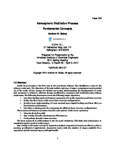
by the three points .1; 0; 0/, .0; 1; 0/, and .0; 0; 1/ as corners. The ternary diagram displays this triangle in the drawing plane with the corners annotated by the axis on which this corner lies. This is possible since closed datasets of three parts have only 2 degrees of freedom. Figure 2.2 illustrates this with the MgO,CaO, and Na2 O subcomposition of the example dataset. For the interpretation of ternary diagrams, we can make use of the property that the orthogonal segments joining a point with the three sides of an equilateral triangle (the heights of that point) have always the same total length: the length of each segment is taken as the proportion of a given part. Ternary diagrams have the merit of actually representing the data as what they are: compositional and relative. Geoscientists are particularly used to this kind of representation. Figures 2.3 and 2.4 show several ways in which the relative portions and proportions of the components of a three-part composition can be read from a ternary diagram. It is worth mentioning that when the three parts represented have too different magnitudes, data tend to collapse on a border or a vertex, obscuring the structure:

2 Fundamental Concepts of Compositional Data Analysis

C

0

A +B +C = ) 1

0.1

0.9

0.2

0.8

0.3

0.7

0.4

0.6

0.5

0.5

0.6

0.4

0.7

0.3

0.8

0.2

0.9

0.1

=1 C C) + +B (A

0

26

A

(A

B =0 (A+B+C)

0.1

0.2

0.3

0.4

0.5

0.6

C

0.7

0.8

0.9

1

B

1 0.9 0.8 0.7

0.1

0.2

0.9

0.4

0.5 0.6 0.7 0.8

0.8 1

0.9

0.7

0.3

0.6

1

0.4

0.3

0.2

0.1

0

A

0.5

0.1 0

B

Fig. 2.3 In a ternary diagram, the portion of each part is represented by the portion of the height of the point over the side of the triangle opposite to the part on the total height of the triangle. However, it is difficult to judge height visually. If we assume the three sides of the triangle to form a sequence of axes, we can make a projection of the point onto the axis pointing towards the interesting part parallel to the previous axis. Consequently, a composition on an edge of the triangle only contains the two parts connected by the side, and a composition in a vertex of the triangle will only contain the part the vertex is linked to. Thus, all compositions along a line parallel to an axis have the same portion of the part opposite to the axis

a typical practice here is to multiply each part by a constant and reclose the result. One can obtain a ternary diagram in R by using plot(x), with x an object of any compositional class (acomp or rcomp, see next section for details). > xc = acomp(GeoChemSed, c("MgO","CaO","Na2O")) > plot(xc)

2.3 Elementary Compositional Graphics

27

C

B = 0 0.1 0.2 0.3 0.4 0.5 0.6 0.7 0.8 0.9 1 (A+B)

A

0.1

0.2

0.3

0.4

0.5

0.6

0.7

0.8

0.9

1

A =1 (A+B)

0.9

0.8

0.7

0.6

0.5

0.4

0.3

0.2

0.1

0

B

1 0.9 0 0.8 0.1 0.7 0.2 0.6 0.3 0.5 0.4 0.4 0.5 0.3 0.6 0.2 0.7 0.1 0 0.8 = B ) 0.9 +C 1 (B = C ) +C (B

(A C +C ) =0 (A A 0.1 +C ) =1 0.2 0.9 0.3 0.4 0.8 0.7 0.5 0.6 0.6 0.7 0.5 0.8 0.4 0.3 0.9 0.2 1 0.1 0

B = 0 (A+B)

C

A

B

B =0 (A+B)

0.1

0.2

0.3

0.4

0.5

0.6

0.7

0.8

0.9

1

A =1 (A+B)

0.9

0.8

0.7

0.6

0.5

0.4

0.3

0.2

0.1

0

Fig. 2.4 The two part subcompositions can be read in two ways: (1) by projecting the composition to an edge of the triangle along a ray coming from the vertex of the part that should be ignored. Thus, all compositions along such rays have the same subcomposition, when the part where the ray is coming from is removed. (2) By drawing a scale between 0 and 1 on a segment parallel to the axis opposite to the part we want to remove, passing through our datum

2.3.3 Log-Ratio Scatterplots Log-ratio scatterplots are just scatterplots of the log ratio of two parts against that of two other parts, though sometimes the denominators are the same. This representation is fully coherent with the description of compositions given in Sect. 2.1 but on the other side, does not capture any mass balance between the represented parts. In fact, it is “independent” of such mass balances: whenever we

28

2 Fundamental Concepts of Compositional Data Analysis

−1.5

log(TiO2/K2O)

−2.0

−2.5

−3.0

−3.5

2.0

2.2

2.4

2.6

2.8

3.0

log(CaO/P2O5)

Fig. 2.5 Example of a log-ratio scatter plot obtained using the formula interface. This example was obtained with plot(log(TiO2/K2O) log(CaO/P2O5),GeoChemSed). Recall that the formula syntax is y  x

cannot ensure that the studied system is not shrinking or growing, then log ratios of scatterplots display almost all the information we really have. For instance, if we are working with transported sediments, we do not know if any part can be dissolved by water and removed from the system; or when dealing with party vote shares between two different elections, we do not know if exactly the same people took part in the election. In fact, most of the datasets obtained in natural systems (meaning, not in the lab under strictly controlled situations) will be in such situations. Despite these issues, scatterplots of log ratios are seldom encountered in applications. To generate a log-ratio scatterplot, one can use the formula interface to plot(formula, data), providing the data set where the variables involved will be extracted, and the desired formula describing the log ratios: > plot(log(var1/var2)~log(var3/var4), dataset) > plot(I(var1/var2)~I(var3/var4), dataset, log="xy") Figure 2.5 shows an example obtained with the first syntax. These two syntax examples would only differ in the way axes are labeled, with the transformed values in the first case, with the original values of the ratios in the second case (using the command I is needed to tell R that the quotient inside it are not symbolic formulae, but actual ratios).

2.3.4 Bar Plots and Pie Charts A bar plot is a classical representation where all parts may be simultaneously represented. In a bar plot, one represents the amount of each part in an individual as a bar within a set. Ideally, the bars are stacked, with heights adding to the total of the composition (1 or 100 %). Then, each individual is represented as one of such

2.4 Multivariate Scales

29

wheat

1.0 Other Protein Carbonates Fat

0.8

Carbonates

0.6 Fat

0.4 Other

0.2

0.0

Protein

soy

wheat

beans

Fig. 2.6 Examples of bar plot (left) and pie plot (right). Note the presence of an extra segment on top of the bars for beans, showing the presence of a missing value

stacked bars, possibly ordered if that is possible (e.g., in time series). Stacked bars are provided in R by the command barplot(x), when x is a compositional dataset. Individual compositions can also be displayed in the form of pie charts. Pie charts are produced by the pie(x) command, but now x must be a single composition (as only one pie diagram will be generated). Pie charts are not recommended for compositions of more than two parts, because the human eye is weak in the comparison of angles if they are not aligned (Bertin, 1967). Figure 2.6 is created by > barplot( acomp(Amounts),xlim=c(0,11) ) > pie( acomp(Amounts["wheat",]), main="wheat")

2.4 Multivariate Scales A fundamental property of each variable (or set of variables) in a dataset is its scale. The scale of a measurement describes which values are possible outcomes and which mathematical operations on these values are meaningful in the context of the application. Classical statistical practice distinguishes several scales for single variables, like (e.g., Stevens, 1946): categorical (several values are possible, but they are not comparable), ordinal (several values are possible, and they can be compared by ordering them), interval (any value in a subset of the real line is a possible outcome, absolute differences between them are meaningful), and ratio (any value in a subset of the positive real line is a possible outcome, relative differences between them matter). Other authors have criticized this list for being too limited: for instance, it does not include a separation between finite, infinite countable, and infinite uncountable scales (in any case, with interval or ratio differences). Although a scale is above all a set of possible values together with some meaningful mathematical operations (and not a statistical model), each scale has

30

2 Fundamental Concepts of Compositional Data Analysis

typical statistical models associated to them: e.g., the multinomial distribution is the most adequate and general model for categorical data, and the normal distribution appears as a central distribution for the real interval scale. Compositional data add a further complexity to the scale issues as they are multivariate objects on themselves. In a composition, we cannot treat one isolated variable because its values are only meaningful in relation to the amounts of the other variables. The whole composition has thus to be considered as a unique object with some scale with joint properties, such as summing to 1 or 100 %, being positive, and obeying a ratio law of difference. A compositional scale is thus a new multivariate scale, not just the concatenation of several separate scales for each variable. Compositional data has historically been treated in several ways according to different considerations on the underlying scale, and there was a lot of discussion on which is the right way of doing so. The “compositions” package provides several of these alternative approaches, with the aim of facilitating the comparison of results obtained following each of them. However, from our experience and the considerations presented in the first sections of this chapter, one of these scales should be the preferred one, as it is the one grounded in the mildest hypotheses: this is the Aitchison (1986) geometry for compositions, discussed in Sect. 2.5. Therefore, this book focuses on this scale, and the next section will introduce it in detail. But depending on our view of the problem, in some case, other scales might be more appropriate. They are available in the package and thus all presented and briefly discussed in this section for the sake of completeness. A comprehensive treatment of the multiple scale mechanisms in the package can be found in van den Boogaart and Tolosana-Delgado (2008). To highlight the relevance of the choice of a scale, in “compositions”, you assign it to the dataset before any analysis. This is done by a command like (e.g., acomp for Aitchison Composition): DataWithScale data(quakes) > MultivariateData data(phosphor) > x data(iris) > x data(Hydrochem) > dat class(dat) [1] "acomp" Further analysis of dat will then be automatically performed in a way consistent with the chosen compositional scale.

2.5 The Aitchison Simplex

37

2.5 The Aitchison Simplex 2.5.1 The Simplex and the Closure Operation A composition which elements sum up to a constant is called a closed composition, e.g., resulting from applying the closure operation (2.1). With “compositions”, you can close a vector or a dataset using the command clo. The set of possible closed compositions ( S WD

x D .xi /i D1;:::;D W xi  0;

D

( D

D X

) xi D 1

i D1

x D .x1 ; : : : ; xD / W xi  0;

D X

) xi D 1

i D1

is called the D-part simplex. Throughout the book, notations x, .xi /i , .x1 ; : : : ; xD / and .xi /i D1;:::;D will equivalently be used to denote a vector, in the two last cases showing how many components it has. The first two notations are reserved for cases where the number of components is obvious from the context or not important. There is some discussion on whether the parts should be allowed to have a zero portion (xi D 0) or not. For the scope of this book, zero values will be considered special cases, pretty similar to missing values (see Chap. 7). The simplex of D D 3 parts is represented as a ternary diagram, where the three components are projected in barycentric coordinates (Sect. 2.3.2). In the same way, the simplex of D D 4 parts can be represented by a solid, regular tetrahedron, where each possible 3-part composition is represented on one side of the tetrahedron. To represent a given 3-part subcomposition of a 4-part dataset, we can project every 4-part datum inside the tetrahedron onto the desired side with projection lines passing through the opposite vertex, corresponding to the removed part. This is exactly the same as closing the subcomposition of the three parts kept. With help of that image, we can conceive higher-dimensional simplexes as hyper-tetrahedrons which projections onto 3- or 4-part sub-simplexes give ternary diagrams and tetrahedral diagrams.

2.5.2 Perturbation as Compositional Sum The classical algebraic/geometric operations (addition/translation, product/scaling, scalar product/orthogonal projection, Euclidean distance) used to deal with conventional real vectors are neither subcompositionally coherent nor scaling invariant. As an alternative, Aitchison (1986) introduced a set of operations to replace these conventional ones in compositional geometry. Perturbation plays the role of sum or translation and is a closed component-wise product of the compositions involved:

38

2 Fundamental Concepts of Compositional Data Analysis

z D x˚y D C Œx1  y1 ; : : : ; xD  yD :

(2.2)

With “compositions”, one can perturb a pair of compositions in two ways: by using the command perturbe(x,y) or by adding or subtracting two vectors of class acomp, i.e., >

(x = acomp(c(1,2,3)))

[1] 0.1667 0.3333 0.5000 attr(,"class") [1] acomp >

(y = acomp(c(1,2,1)))

[1] 0.25 0.50 0.25 attr(,"class") [1] acomp >

(z = x+y)

[1] 0.125 0.500 0.375 attr(,"class") [1] acomp The neutral element of perturbation is the composition ½ D Œ1=D; : : : ; 1=D. It is an easy exercise to show that for any composition x, the neutral elements fulfill x˚½ D x. The neutral element is thus playing the role of the zero vector. Any composition x D Œx1 ; : : : ; xD  has its inverse composition: if one perturbs both, the result is always the neutral element. The inverse is x D C Œ1=x1 ; : : : ; 1=xD  and it holds x ˚ x D . Perturbation by the opposite element plays the role of subtraction, hence the notation with . Perturbation with an inverse composition can as usually also be denoted with a binary  operator: x  y WD x ˚ y. In “compositions”, inverse perturbation can be obtained subtracting two compositions, x-y or with perturbe(x,-y).

Example 2.2 (How and why do we perturb a whole dataset?). To perturb a whole compositional dataset by the same composition, we have to give both objects an acomp class and just ask for the dataset plus (or minus) the composition, for instance, > > > > > >

data(Hydrochem) Xmas = Hydrochem[,c("Cl","HCO3","SO4")] Xmas = acomp(Xmas) mw = c(35.453, 61.017, 96.063) mw = acomp(mw) Xmol = Xmas-mw

2.5 The Aitchison Simplex

39

D Xmas contains the subcomposition Cl –HCO 3 –SO4 in mass proportions, and this is recasted to molar proportions in Xmol by dividing each component (inverse perturbation) with its molar weight (in mw). Most changes of compositional units may be expressed as a perturbation (between molar proportions, mass percentages, volumetric proportions, molality, ppm, etc.), as explained in Sect. 2.2.2. This operation is also applicable in the centering procedure of Sect. 4.1. Note that the two involved objects must have either the same number of rows (resulting in the perturbation of the first row of each dataset, the second of each dataset, etc.) or one of them must have only one row (resulting in all rows of the other object perturbed by this one).

In statistical analysis, it is often necessary to perturb or “sum up” all the compositions in the dataset. This is denoted by a big ˚: n M

xi WD x1 ˚ x2 ˚    ˚ xn

i D1

2.5.3 Powering as Compositional Scalar Multiplication Powering or power transformation replaces the product of a vector by a scalar (geometrically, this is equivalent to scaling) and is defined as the closed powering of the components by a given scalar:  z D ˇx D C Œx1 ; : : : ; xD :

(2.3)

Again, the package offers two ways to power a composition by a scalar: with the generic function power(x,y) or by multiplying a scalar by a vector of class acomp. > 2*y [1] 0.1667 0.6667 0.1667 attr(,"class") [1] acomp

2.5.4 Compositional Scalar Product, Norm, and Distance The Aitchison scalar product for compositions hx; yiA D

D 1 X xi yi ln ln D i >j xj yj

(2.4)

40

2 Fundamental Concepts of Compositional Data Analysis

provides a replacement for the conventional scalar product. The generic function scalar(x,y) has been added to “compositions” to compute scalar products: if x and y are acomp compositions, the result will be that of (2.4). Recall that the scalar product induces a series of secondary, useful operations and concepts. p • The norm of a vector, its length, is kxkA D hx; xiA . From an acomp vector x, its norm can be obtained with norm(x). If x is a data matrix of class acomp, then the result of norm(x) will be a vector giving the norm of each row. • The normalized vector of x (or its direction, or a unit-norm vector) is v D kxk1 A ˇx. The generic function normalize provides this normalization, either for a single composition or for the rows of a data matrix. • The angle between two compositions, ˛.x; y/ D cos1

˝ ˛ hx; yiA 1 D cos1 kxk1 A ˇx; kykA ˇy A ; kxkA  kykA

which allows to say that two compositions are orthogonal if their scalar product is zero, or their angle is 90ı . This is not implemented in a single command, but you get it with > acos(scalar(normalize(x),normalize(y))) • The (orthogonal) projection of a composition onto another is the composition Px .y/ D

hy; xiA ˇx; hx; xiA

or in case of projecting onto a unit-norm composition, Pv .y/ D hy; viA ˇv. This last case appears next when discussing coordinates with respect to orthonormal bases. A related concept is the (real) projection of a composition on a given direction, hy; viA , which is a single real number. • The Aitchison distance (Aitchison, 1986) between two compositions is v u  D  D X u1 X xi yi 2 t dA .x; y/ D kx  x; ykA D ln  ln : D i D1 j >i xj yj

(2.5)

The distance between two compositions can be directly computed by norm(x-y).

In “compositions”, the generic function dist automatically computes the Aitchison distances between all rows of an acomp data matrix. The result is an object of class dist, suitable for further treatment (e.g., as input to hierarchical cluster analysis, see Sect. 6.2). Note that other compositional

2.5 The Aitchison Simplex

41

distances, like Manhattan or Minkowski distances, are also available through the extra argument method: > > > > >

a = acomp(c(1,2,4)) b = acomp(c(3,3,1)) mycomp = rbind(a,b) mycomp = acomp(mycomp) dist(mycomp)

a b 1.813 > norm(a-b) [1] 1.813 > dist(mycomp,method="manhattan") a b 2.851 > sum(abs(clr(a-b))) [1] 2.851

2.5.5 The Centered Log-Ratio Transformation (clr) The set of compositions together with the operations perturbation ˚, powering ˇ and Aitchison scalar product .; /A build a .D  1/-dimensional Euclidean space structure on the simplex. This means that we can translate virtually anything defined for real vectors to compositions, as an Euclidean space is always equivalent to the real space. This equivalence is achieved through an isometry, i.e., a transformation from the simplex to the real space that keeps angles and distances. The first isometric transformation we use is the centered log-ratio transformation (clr)   xi clr.x/ D ln g.x/ i D1;:::;D

with

g.x/ D

p D x1  x2    xD ;

(2.6)

or in a compact way clr.x/ D ln.x=g.x//, where the log ratio of the vector is applied component-wise. The inverse clr transformation is straightforward: if x D clr.x/, then x D C Œexp.x /, where the exponential is applied by components. By its definition, the clr transformed components sum up to zero: in fact, the image of

42

2 Fundamental Concepts of Compositional Data Analysis

Fig. 2.7 Representation of a 3-part simplex (ABC, S3 ) and its associated clr-plane (H), with an orthogonal basis  3 fv 1 ; v2 ; v3 g of R . The reader can find illustrative to play with a 3-D representation of the clr-transformed data of a 3-part composition, like > > > > >

data(Hydrochem) idx = c(14,17,18) x = Hydrochem[,idx] x = acomp(x) plot3D(x, log=TRUE)

the clr is a hyperplane (and a vector subspace, denoted with H, called the clr-plane) of the real space H  RD orthogonal to the vector 1 D Œ1; : : : ; 1, i.e., the bisector of the first orthant (Fig. 2.7). This may be a source of problems when doing statistical analyses, as e.g., the variance matrix of a clr-transformed composition is singular. The commands clr and clrInv compute these two transformations: they admit either a vector (considered as a composition), or a matrix or data frame (where each row is then taken as a composition).

2.5.6 The Isometric Log-Ratio Transformation (ilr) It is well known that there is only one .D1/-dimensional Euclidean space typically called RD1 , up to an isometric mapping. Therefore, there exist an isometric linear mapping between the Aitchison simplex and RD1 . This mapping is called the isometric log-ratio transformation (ilr). The isometry is constructed by representing the result in a basis of the .D  1/dimensional image space H of the clr transformation. This is constructed by taking an orthonormal basis of RD including the vector vD D Œ1; : : : ; 1, i.e., some .D  1/ linearly independent vectors fv1 ; : : : ; vD1 g 2 H (Fig. 2.7). Then the set of compositions defined as vi D clr1 .vi / form a basis of SD . In computational terms, one can arrange the vectors fvj g by columns in a D  .D  1/-element matrix, denoted by V, with the following properties: • It is a quasi-orthonormal matrix, as Vt  V D ID1

and V  Vt D ID 

1 1DD ; D

(2.7)

2.5 The Aitchison Simplex

43

where ID is the D  D identity matrix, and 1DD is a D  D matrix full of ones. • Its columns sum up to zero, because they represent vectors of the clr-plane, 1  V D 0:

(2.8)

Thanks to these properties, we can find simple expressions to pass between coordinates  and compositions x: clr.x/  Vt D ln.x/  Vt DW ilr.x/ D 

(2.9)

ilr.x/  V D clr.x/ ! x D C Œexp .  V/ :

(2.10)

Through these expressions, we also defined implicitly the so-called isometric logratio transformation (ilr): this is nothing else than a transformation that provides the coordinates of any composition with respect to a given orthonormal basis. There are as many ilr as orthonormal basis can be defined, thus as matrices V fulfilling (2.7) and (2.8). The one originally defined by Egozcue et al. (2003) was based on the (quite ugly) Helmert matrix 1 0 D1 p 0  0 0 D.D1/ C B p 1 D2  0 0 C B D.D1/ p.D1/.D2/ C B 1 1 C Bp B D.D1/ p.D1/.D2/    0 0 C B :: :: : : :: :: C (2.11) VDB : : : C : : C: B C B 1 2 1 p Bp    p6 0 C C B D.D1/ .D1/.D2/ B p 1 1 1 C 1 @ D.D1/ p.D1/.D2/    p6 p2 A 1 p 1 1 p 1 p  p D.D1/ .D1/.D2/ 6

2

The ilr transformation induces an isometric identification of RD1 and SD . For measure and probability theory purposes, this induces an own measure for the simplex, called the Aitchison measure on the simplex, denoted as S , and completely analogous to the Lebesgue-measure . This Aitchison measure is given by S .A/ D .filr.x/ W x 2 Ag/:

The ilr transformation is available through the command ilr(x). An optional argument V can be used to specify a basis matrix different from the default one. This is itself available through the function ilrBase(x,z,D), where the arguments represent, respectively, the composition, its ilr transformation, and its number of parts (only one of them can be passed!). An alternative interface to some ilr transformations is provided by the functions balance(x) and balanceBase(x), explained in Sect. 4.3. The commands ilrInv provide the inverse transformation. Also, if we want to pass from ilr to clr or vice versa, we can use functions ilr2clr and clr2ilr.

44

2 Fundamental Concepts of Compositional Data Analysis

> a = c(1,2,4) > (ac = acomp(a)) [1] 0.1429 0.2857 0.5714 attr(,"class") [1] acomp > ilr(ac) [,1] [,2] [1,] 0.4901 0.8489 attr(,"class") [1] "rmult" > clr2ilr(clr(ac)) [1] 0.4901 0.8489 > (Vd = ilrBase(x=a)) [,1] [,2] 1 -0.7071 -0.4082 2 0.7071 -0.4082 3 0.0000 0.8165 > clr(ac) %*% Vd [1] 0.4901 0.8489 attr(,"class") [1] "rmult"

2.5.7 The Additive Log-Ratio Transformation (alr) Finally, it is worth mentioning that compositional data analysis in the original approach of Aitchison (1986) was based on the additive log-ratio transformation (alr), alr.x/ D .ln.x1 =xD /; : : : ; ln.xD1 =xD // D .ln.xi =xD //i D1;:::;D1 . Though we will not use it in this book, the alr transformation is available with the command alr(x).

Remark 2.2 (Why so many log-ratio transformations?). The answer is quite easy: because none is perfect. All three of them recast perturbation and

2.5 The Aitchison Simplex

45

powering to classical sum and product, clr.x˚y/ D clr.x/ C clr.y/; ilr.x˚y/ D ilr.x/ C ilr.y/; alr.x˚y/ D alr.x/ C alr.y/ clr.ˇx/ D   clr.x/; ilr.ˇx/ D   ilr.x/; alr.ˇx/ D   alr.x/: The first two, because they are isometric, also preserve the scalar product, but this does not happen with the alr transformation, hx; yiA D clr.x/  clrt .y/ D ilr.x/  ilrt .y/ ¤ alr.x/  alrt .y/ Thus, alr should not be used in case that distances, angles, and shapes are involved, as it deforms them. On the other side, we already mentioned that the clr yields singular covariance matrices, and this might be a source of problems if the statistical method used needs inverting it. One would need to use Moore–Penrose generalized inverses. As an advantage, the clr represents a one-by-one link between the original and the transformed parts, which seems to be helpful in interpretation. This is exactly the strongest difficulty with the ilr-transformed values or any orthonormal coordinates: each coordinate might involve many parts (potentially all), which makes it virtually impossible to interpret them in general. However, the ilr is an isometry and its transformed values yield full-rank covariance matrices; thus, we can analyze ilr data without regard to inversion or geometric problems. The generic ilr transformation is thus a perfect black box: compute ilr coordinates, apply your method to the coordinates, and recast results to compositions with the inverse ilr. If interpretation of the coordinates is needed, one should look for preselected bases and preselected ilr transformations, as those presented in Sect. 4.3.

2.5.8 Geometric Representation of Statistical Results The fact that the simplex is an Euclidean space has some implications on the way we apply, interpret and represent most linear statistics. The basic idea is summarized in the principle of working on coordinates (Pawlowsky-Glahn, 2003), stating that one should: 1. Compute the coordinates of the data with respect to an orthonormal basis (2.9).

46

2 Fundamental Concepts of Compositional Data Analysis

2. Analyze these coordinates in a straightforward way with the desired method; no special development is needed, because the coordinates are real unbounded values. 3. Apply those results describing geometric objects to the orthonormal basis used, recasting them to compositions (2.10). Final results will not depend on the basis chosen. Regarding the last step, most “geometric objects” obtained with linear statistics are points or vectors, lines/hyperplanes, and ellipses/ellipsoids. Points (like averages and modes or other central tendency indicators, outliers, intersection points, etc.) are identified with their vectors of coordinates in the basis used. Thus, to represent a point as a composition, it suffices to apply its coordinates to the basis, i.e., compute the inverse ilr transformation (2.10). To draw points in a ternary diagram (or a series of ternary diagrams), one can use the function plot(x) where x is already a composition of class acomp (or a dataset of compositions). If points have to be added to an existing plot, the optional argument add=TRUE will do the job. This function admits the typical R set of accessory plotting arguments (to modify color, symbol, size, etc.). Lines (like regression lines/surfaces, principal components, discriminant functions, and linear discriminant borders) are completely identified with a point ˛ and a vector ˇ in the clr-plane. The parametric equation .t/ D ˛Ct ˇ runs through every possible point of the line taking different values of the real parameter t. Applying this parametric equation to the basis in use, we obtain a compositional line, x.t/ D a˚tˇb;

(2.12)

with a D ilr1 .˛/ and b D ilr1 .ˇ/. A P -dimensional plane needs P compositions of the second kind, i.e., MP ti ˇbi : x.t1 ; : : : ; tP / D a˚ i D1

(2.13)

Note that a P -dimensional plane projected onto a subcomposition is still a P -dimensional plane. In particular, a line projected on a 3-part subcomposition is a line, obtained by selecting the involved parts in the vectors a and b. Straight lines can be added to existing plots by the generic function straight(x,d), which arguments are respectively the point a and the vector b (as compositions!). Sometimes only a segment of the line is desired, and two functions might be helpful for that. Function segments(x0,y) draws a compositional line from x0 to y, i.e., along y-x0; both can be compositional datasets, thus resulting in a set of segments joining x0 and y row by row. Function lines(x) on the contrary needs a compositional dataset and draws a piece-wise (compositional) line through all the rows of x. Further graphical arguments typical of lines (width, color, style) can also be given to all these functions. Ellipses and hyper ellipsoids (like confidence or probability regions or quadratic discriminant borders) are completely specified by giving a central point ˛ and a

2.5 The Aitchison Simplex

47

symmetric positive definite matrix T. An ellipse is the set of points  fulfilling .  ˛/  T  .  ˛/t D r 2 ;

(2.14)

namely, the set of points with norm r by the scalar product represented by the matrix T. This can be extended to conics (and hyper quadrics) by dropping the condition of positive definiteness. Any hyper quadric projected onto a subcomposition is still a hyper quadric. In particular, in two dimensions (three parts), an ellipse is obtained with a positive definite matrix, a parabola with a semi-definite matrix, and an hyperbola with a non-definite matrix. All hyper quadrics show up as borders between subpopulations in quadratic discriminant analysis. But by far, their most typical use is to draw elliptic probability or confidence regions around the mean (see Example 4.2). In this case, we can better characterize the ellipses with the original variance matrix, i.e., T D S1 . This is the approach implemented in the generic function ellipses(mean, var, r), which arguments are a central composition (mean), a clr-variance matrix (var, described in Sect. 4.1), and the radius of the ellipse (r). Further graphical arguments for lines are also admitted.

Summary of graphical functions: • plot(x) to draw ternary diagrams of the acomp composition x • plot(x, add=TRUE) to add compositions to existing ternary diagrams • straight(x,d) to draw lines on ternary diagrams along d passing through x, both acomp compositions – segments(x0,y) to add compositional segments from the rows of x0 to the rows of y – lines(x) to add piece-wise compositional lines through x rows • ellipses(mean, var, r) to draw an ellipse around the acomp composition mean, defined by a radius r and a clr-variance var

2.5.9 Expectation and Variance in the Simplex In an Euclidean space, like the simplex, expectation and variance can be defined with regard to its geometry. Eaton (1983) presents the theory for any Euclidean space, and we will here present without proof the most important results in the Aitchison geometry of the simplex. The goal of this section is twofold. On the one hand, we want to see that the actual basis used to compute coordinates and apply statistics is absolutely irrelevant: back-transformed results are exactly the same whichever basis

48

2 Fundamental Concepts of Compositional Data Analysis

was used. On the other hand, we will also find that variance matrices may be seen as representations of some objects on themselves, with a full meaning: this ensures us that whichever log-ratio transformation we use (clr, ilr or alr), expressions like (2.14) are fully correct as long as all vectors and matrices are obtained with regard to the same log-ratio transformation. Take the Euclidean space structure of the simplex .SD ; ˚; ˇ; h; iA / and a random composition X 2 SD . Its expectation within the simplex is a fixed composition m such that the expected projection of any composition v 2 SD onto X is perfectly captured by its projection onto m, ES ŒX D m , for all v W E Œhv; XiA  D hv; miA :

(2.15)

This says that knowing m, we know the average behavior of X projected onto any direction of the simplex. This definition does not make use of any basis, so we can be sure that the concept itself is basis-independent. To compute it, however, we may take the vector v successively as each of the .D  1/ vectors of any ilr basis, thus obtaining the mean coordinates with respect to that basis, ilr .ES ŒX/ D EŒilr.X/ 2 RD1 This is the result we would obtain by applying the principle of working on coordinates. In other words, the definition given by (2.15) and the one implied by the principle of working on coordinates are equivalent, and both are in fact basisindependent. For the variance, we may obtain equivalent results by defining it as an endomorphism. An endomorphism within the simplex is an application ˙ W SD ! SD that preserves the linearity of perturbation and powering, e.g., ˙.x˚ˇy/ D ˙.x/˚ˇ˙.y/. The variance within the simplex of a random composition X 2 SD is an endomorphism ˙ such that the expected product of the projections of any pair of compositions u; w 2 SD onto X (centered) is perfectly captured by their scalar product through ˙: varS ŒX D ˙ ) E Œhw; X  miA  hu; X  miA  D hw; ˙.u/iA D hu; ˙.w/iA : (2.16) In words, by knowing ˙, we know the expected covariation of X projected onto any pair of directions of the simplex. As with expectation, the ilr-coordinate representation of ˙ is a .D  1/  .D  1/ matrix ˙ v D .ijv / such that ijv D covŒilri .X/; ilrj .X/. And equivalently, its clr representation is a D  D matrix ˙ D .ij / such that ijv D covŒclri .X/; clrj .X/. Note that, whichever transformation we use, hu; ˙.w/iA D .ilr.u/; ilr.˙.w/// D ilr.u/  ˙ v  ilrt .w/ D clr.u/  ˙  clrt .w/:

References

49

Thus, all these matrices and vectors, expressed as compositions, in clr coefficients or in ilr coordinates, represent exactly the same objects. We can consistently change between them with the following expressions: ilr.m/ D clr.m/  V D v ˙ v D Vt  ˙  V

m D clr1 .v  Vt / D ilr1 .v /; ˙ D V  ˙ v  Vt :

(2.17)

Functions clrvar2ilr(xvar) and ilrvar2clr(zvar) implement the variance transformations of (2.17), where xvar is the clr variance ˙ and zvar is the ilr variance ˙ v . To transform the mean vector, we may use the self-explaining functions ilr, clr, ilrInv, clrInv, ilr2clr, and clr2ilr.

References Aitchison, J. (1981). Distributions on the simplex for the analysis of neutrality. In C. Taillie, G. P. Patil, & B. A. Baldessari (Eds.), Statistical distributions in scientific work—Models, structures, and characterizations (pp. 147–156). Dordrecht: D. Reidel Publishing Co., 455 pp. Aitchison, J. (1986). The statistical analysis of compositional data. Monographs on statistics and applied probability. London: Chapman & Hall (Reprinted in 2003 with additional material by The Blackburn Press), 416 pp. Aitchison, J. (1997). The one-hour course in compositional data analysis or compositional data analysis is simple. In V. Pawlowsky-Glahn (Ed.), Proceedings of IAMG’97—The third annual conference of the International Association for Mathematical Geology, Volume I, II and addendum (pp. 3–35). Barcelona: International Center for Numerical Methods in Engineering (CIMNE), 1100 pp. Aitchison, J., & Egozcue, J. J. (2005). Compositional data analysis: Where are we and where should we be heading? Mathematical Geology, 37(7), 829–850. Barcel´o-Vidal, C. (2000). Fundamentaci´on matem´atica del an´alisis de datos composicionales. Technical Report IMA 00-02-RR. Spain: Departament d’Inform´atica i Matem´atica Aplicada, Universitat de Girona, 77 pp. Bertin, J. (1967). Semiology of graphics. Madison: University of Wisconsin Press. Billheimer, D., Guttorp, P., & Fagan, W. (2001). Statistical interpretation of species composition. Journal of the American Statistical Association, 96(456), 1205–1214. Butler, J. C. (1978). Visual bias in R-mode dendrograms due to the effect of closure. Mathematical Geology, 10(2), 243–252. Butler, J. C. (1979). The effects of closure on the moments of a distribution. Mathematical Geology, 11(1), 75–84. Chayes, F. (1960). On correlation between variables of constant sum. Journal of Geophysical Research, 65(12), 4185–4193. Chayes, F., & Trochimczyk, J. (1978). An effect of closure on the structure of principal components. Mathematical Geology, 10(4), 323–333. Cortes, J. A. (2009). On the Harker variation diagrams; a comment on “the statistical analysis of compositional data. Where are we and where should we be heading?” by Aitchison and Egozcue (2005). Mathematical Geosciences, 41(7), 817–828. Eaton, M. L. (1983). Multivariate statistics. A vector space approach. New York: Wiley. Egozcue, J. J., Pawlowsky-Glahn, V., Mateu-Figueras, G., & Barcel´o-Vidal, C. (2003). Isometric logratio transformations for compositional data analysis. Mathematical Geology, 35(3), 279–300.

50

2 Fundamental Concepts of Compositional Data Analysis

Pawlowsky-Glahn, V. (1984). On spurious spatial covariance between variables of constant sum. Science de la Terre, S´erie Informatique, 21, 107–113. Pawlowsky-Glahn, V. (2003). Statistical modelling on coordinates. In S. Thi´o-Henestrosa & J. A. Mart´ın-Fern´andez (Eds.), Compositional data analysis workshop—CoDaWork’03, Proceedings. Catalonia: Universitat de Girona. ISBN 84-8458-111-X, http://ima.udg.es/Activitats/ CoDaWork03/. Pawlowsky-Glahn, V., & Egozcue, J. J. (2001). Geometric approach to statistical analysis on the simplex. Stochastic Environmental Research and Risk Assessment (SERRA), 15(5), 384–398. Pawlowsky-Glahn, V., Egozcue, J. J., & Burger, H. (2003). An alternative model for the statistical analysis of bivariate positive measurements. In J. Cubitt (Ed.), Proceedings of IAMG’03—The ninth annual conference of the International Association for Mathematical Geology (p. 6). Portsmouth: University of Portsmouth. Pearson, K. (1897). Mathematical contributions to the theory of evolution. On a form of spurious correlation which may arise when indices are used in the measurement of organs. Proceedings of the Royal Society of London, LX, 489–502. Shurtz, R. F. (2003). Compositional geometry and mass conservation. Mathematical Geology, 35(8), 927–937. Stevens, S. (1946). On the theory of scales of measurement. Science, 103, 677–680. Tolosana-Delgado, R., & von Eynatten, H. (2010). Simplifying compositional multiple regression: Application to grain size controls on sediment geochemistry. Computers and Geosciences, 36, 577–589. van den Boogaart, K. G., & Tolosana-Delgado, R. (2008). “compositions”: A unified R package to analyze compositional data. Computers and Geosciences, 34(4), 320–338.

http://www.springer.com/978-3-642-36808-0