Chapter 16: Empirical Evidence on Demand, Supply and Surpluses 16.1: Introduction This chapter shows that the theoretical material that we have been studying has empirical relevance. We apply the theory to the estimation of a demand and supply system for some commodity. We are searching for a specification that has both theoretical justification and fits the facts - is empirically relevant. If you want, you can reproduce what we have done here with other commodities. We should warn you that this chapter assumes some basic familiarity with basic econometrics particularly the concept of a regression. If you have not yet done any econometrics, full understanding of this chapter may have to wait until later. I thought about including some material on econometric pre-requisites, but decided on the grounds that such material would take up too much space. There is however a glossary of key terms at the end of the chapter. If you really have not done any basic regression analysis before, I would suggest that you reserve this chapter for a later date, and take on faith the important message: that the theory we are presenting in this book does have empirical relevance and is useful. I should note that nothing in the rest of the book relies on you understanding (or even having read) this chapter.

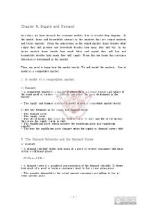
16.2: The data to be explained The data that we are using is reproduced at the end of this chapter. We choose a commodity that is important and interesting - the demand for and supply of food in the UK. We need to start with some data. This we obtained from the publication Economic Trends Annual Supplement (ETAS). (Actually the data was downloaded electronically from the UK Data Archive which is located at the University of Essex, but the data is also available in printed format in ETAS.) If you look in that publication there are two series for Household Expenditure on Food one series in current prices (code name in ETAS: CCDW) and the other a series in constant 1995 prices (code name CCBM). The first of these is money expenditure while the second corrects for price changes. So it is the latter that is the indicator of the quantity of food purchased. We shall call this variable RFOD - standing for Real expenditure on FOOD. We shall call the variable giving the expenditure on food in current prices NFOD – standing for Nominal expenditure on FOOD. You will find the data on these variables in the table at the end of this chapter – in the 5th and 6th columns of that table. From these two series we can derive the Price of FOOD - which we denote by PFOD – we do this by dividing the series of expenditure on food in current prices by the series of expenditure on food in constant prices. Thus PFOD = NFOD/RFOD. There is data available from 1948 to 1999 - a total of 52 observations. If we draw a scatter diagram of price (PFOD) against quantity (RFOD) we get figure 16.1.

We should note that this is annual data and that each cross represents the price and quantity of food purchased in a particular year. There are 52 observations and hence 52 crosses. The figure looks a little like a supply curve. Note, however, that we have done something odd - since all prices are rising through time we ought to correct the price series for the general movement in prices. We can do this by first obtaining data on overall prices. We do this by taking the series for the total household expenditure in current prices (code name ABPB) - which we shall call NALL (Nominal expenditure on ALL commodities) and dividing it by the total household expenditure in constant prices (code name ABPF) - which we shall call RALL (Real expenditure on ALL commodities). The data on these variables is in the 3rd and 4th columns of the table at the end of this chapter. Dividing NALL by RALL gives us PALL - the Price of ALL commodities. Thus PALL = NALL/RALL. We can then find the relative price of food - PFOD/PALL. Graphed against the quantity of food purchased over the period from 1948 to 1999 we get the scatter diagram in figure 16.2. Again there are 52 crosses – one for each year.

16.3: The demand for food in the UK

Figure 16.2 looks like a demand curve. It looks vaguely linear and perhaps a linear demand curve would be a good fit. But we should think about the theory that we have been studying. Clearly we can reject the hypothesis that food is a perfect substitute for other commodities (you should ask yourself why) and that food is a perfect complement with other commodities (again you should ask yourself why). Let us try Cobb-Douglas preferences. You will recall that this is particularly simple: it states that the amount spend on a commodity is a constant fraction of income. This means that RFOD should be a constant fraction of NALL/PFOD. That is, real expenditure on food should be a constant fraction of the real income (or real total expenditure). Here, for simplicity, we are assuming that the decision taken by the consumer is how to decide the allocation of total consumption over the various commodities - we are taking out the saving decision, which we have not yet studied. If we do a regression of RFOD against NALL/PFOD we get the following: RFOD = 0.146 NALL/PFOD + u (21.0)

log-likelihood = -568.056

This is the equation of the ‘best-fitting’ straight line to the scatter produced by plotting RFOD against NALL/PFOD. You should note that this is not figure 16.2, but you could draw the scatter diagram yourself using the data in the appendix and inserting on the graph the line above. The term in brackets under the coefficient is the t-ratio. The coefficient is clearly significantly different from zero. This coefficient (on NALL/PFOD) indicates that consumers on average spend 14.6% of their total consumption expenditure on food. This is much higher than is actually the case (in 1999 the proportion was less than 10%) - which suggests that the specification is not particularly good. Actually a more direct test of the hypothesis that preferences are Cobb-Douglas can be found by simply looking at the proportion of total expenditure that goes on food: this started out at almost 30% in 1950 but was less than 10% in 1999 – a clear rejection of the Cobb-Douglas specification. The log-likelihood is a measure of the goodness of fit of the equation. The fit is quite good. However it will become clear that other specifications fit the data better. One possible contender is the Stone-Geary Utility function which we know (see equation 7.3 in chapter 7) leads to a demand function of the form: q1 = s1 + a (m – p1s1 – p2s2)/p1 where good 1 is the good of interest (in this case food) and good 2 is all other goods. Let us denote the price of all other goods by QFOD ( which is simply given by (NALL-NFOD)/(RALL-RFOD). Then we can conclude that the Stone-Geary demand function for food is such that RFOD is a linear function of NALL/PFOD and QFOD/PFOD. (That is, using the original notation q1 is a linear function of m/p1 and p2/p1.) If we fit the data to this function we get the following result: RFOD = 44491 + 0.065 NALL/PFOD - 23426 QFOD/PFOD + u (11.4) (10.8) (3.6) log-likelihood = -446.349 R-squared = .94254 residual sum of squares = 86,932,642 The numbers in brackets under the coefficients are the corresponding t-ratios. They clearly are all significant. The implied subsistence level of expenditure on food is £44,491m - equivalent to around £800 per head per year in 1995 prices. The coefficient on the variable NALL/PFOD indicates that once the subsistence levels of both food and other commodities have been bought, consumers on average spend 6.5% of an extra income on food. This seems more reasonable. The log-likelihood of this equation is significantly higher than that for the Cobb-Douglas specification, and the R-squared indicates that 94.2% of the variation in expenditure on food is explained by this

Stone-Geary specification. This specification therefore seems reasonable on econometric grounds1 and on economic grounds.

16.4: Simultaneous bias At this stage we ought to recognise an important fact. The data that we have got on expenditure on food is not just demand data. It is generated by the simultaneous interaction of demand and supply. What effect does this have? We cannot give a full explanation here - a full explanation requires a course in econometrics - but we can explain the nature of the problem. As we have already said, the data that we have results from the interaction of demand with supply. If the demand and supply functions have remained stable throughout the observation period, that must mean that there is only one intersection point - and so we would observe just one value for RFOD and just one value for the price PFOD. As it happens we have lots of different observations - as figures 16.1 and 16.2 make clear. This must imply that one or both of the demand and supply schedules must have moved during the observation period. Let us consider what might have happened. Suppose just the demand schedule has moved. We would have something like figure 16.3.

Notice where the intersection points lie - all along the supply curve! All we can observe from the data is the supply curve. (Notice that we can deduce nothing about the demand curves - just consider a second family of demand curves with slopes different from those above.) If however it was just the supply curve that had moved - we would have something like figure 16.4.

1

We appreciate that econometricians would want to do some further tests of the specification. However such tests are beyond the scope of the book and may require us to bring in some further economic theory. The crucial point is that we have a specification that comes from some economic theory and is econometrically respectable.

Here we would just be able to observe the demand curve. Now we know something from economic theory - we know that changes in income (or changes in the total expenditure) will shift the demand curve and we know that changes in factor prices will shift the supply curve. If we look at data on these variables over the period we are considering we will see that all these variables have indeed changed over the period. So both the demand and supply curve have shifted. If we ignore this information we are going to get biases in our estimation. Going back to the demand curve estimated above, we should recognise that some of the movements must have resulted from shifts in the supply curve. To explain how we eliminate these biases caused by the simultaneous determination of price and quantity takes us deep into econometrics - and we cannot discuss these issues here. Suffice it to say that if we use a method of estimation called Instrumental Variables Estimation (as distinct from Ordinary Least Squares Estimation – which we used above) we can get rid of the bias. Let us report the results of instrumental variables estimation of the demand equation. This method takes into account that the price variable on the right hand side of the equation is partly determined by the variables which enter the supply equation - namely factor prices. Instrumental variables estimation (using the factor prices - which we will discuss later - as instrumental variables) yields the following estimate of the Stone-Geary demand function for food: RFOD = 41962 + 0.049 NALL/PFOD - 14210 QFOD/PFOD + u (8.5) (5.9) (1.6) residual sum of squares = 4,450,094

DEMAND EQUATION

The subsistence level of food expenditure is now £41,962 m in 1995 prices. The proportion of extra income spent on food is 4.9%. You will notice changes in the estimates as a result of the elimination of simultaneous bias through the use of the instrumental variables estimation technique. Given the fact that instrumental variables estimation is a consistent method of estimation while ordinary least squares is not (in the context of a simultaneous system) we take the equation above as out estimate of the demand curve for food in the UK.

16.5: The supply of food in the UK We assume a Cobb-Douglas production function and that the food production industry is competitive. We know from the chapters on cost curves that the cost function for a two-input CobbDouglas is proportional to (see equation (12.1)) y1/(a+b) w1a/(a+b) w2b/(a+b) It follows that the marginal cost function for a firm or an industry with decreasing returns to scale is proportional to y(1-a-b)/(a+b) w1a/(a+b) w2b/(a+b) If we now use the profit maximising condition that price should equal marginal cost and if we solve that equation for the implied optimal output we find that it is given by (where k is some constant) y = k p(a+b)/(1-a-b) w1-a/(1-a-b) w2-b/(1-a-b) This is the supply function for a two-input competitive industry with Cobb-Douglas technology. As most of the econometric packages like linear equations, we linearise it by taking logarithms. We get: log(y) = constant + [(a+b) log(p) – a log(w1) – b log(w2)]/(1-a-b) This is a linear equation in the variables log(y), log(p), log(w1) and log(w2). You will notice that the price of food has a positive coefficient while the input prices all have negative coefficients. Obviously if there are more than 2 factors of production the equation can be generalised appropriately We now need to find some appropriate data. We already have the price of food - PFOD. We restrict attention to variables that can be easily found in Economic Trends Annual Supplement. There are three obvious factors of production - labour, capital and raw materials and fuels. We take as our indicator of the wage rate the variable (code name LNNK in ETAS) Unit Wage Costs in the whole economy (there is no data specifically for the food-producing industry). We call this PUW. We take as our indicator of the cost of capital the Interest rate on long-term government securities. This has the ETAS code AJLX and we call it NLI (the Nominal Long term rate of Interest). Finally, recognising that the food industry has to buy materials and fuel as input we take the price index for raw materials and fuels purchased by manufacturing industry (there is no variable specifically for the food industry). This has ETAS code PLKW and we call it PMAF. The data are listed in the 2nd, 9th and 10th columns of the table at the end of this chapter. Our hypothesis is that the log of RFOD is a linear function of the log of PFOD, the log of PMAF, the log of NLI and the log of PUW. If we carry out an instrumental variables estimation of this equation (again to avoid bias caused by simultaneity) we obtain log(RFOD)= 13.68 + 0.761 log(PFOD) - 0.0948 log (PMAF) - 0.0934 log(NLI) - 0.485 log(PUW) (13.9) (3.3) (1.2) (2.0) (2.1) Residual sum of squares = 0.0102 t-ratios in brackets

SUPPLY EQUATION

This is our estimated supply equation. You will see that all the coefficients have the right sign and are significant - except the coefficient on log(PMAF). We left this in as the ordinary least squares estimation suggested that it was important. For the record the ordinary least squares estimate is reported below: log(RFOD)= 11.98 + 0.348 log(PFOD) - 0.148 log (PMAF) - 0.0696 log(NLI) - 0.0786 log(PUW) (23.5) (3.1) (2.5) (2.0) (0.6) Residual sum of squares = 0.0056 t-ratios in brackets. You might like to disentangle the coefficients of the underlying Cobb-Douglas production function.

16.6: An investigation of the effect of a tax on food At the moment food is exempt from VAT. Suppose the government were considering the imposition of VAT. Let us examine here what would happen. The initial situation is given by the demand and supply equations above. Let us take the position as in 1999 - the latest year for which data is available. In this year we have the following values for the exogenous variables: NALL = 564368

PALL = 1.10043 PMAF = 83.7 NLI = 4.7 PUW = 115 QFOD = 1.10621

If we substitute these values in the demand and supply equations and then graph the demand and supply equations we get figure 16.5.

You will see that the initial equilibrium - a value for RFOD of 52832 and a value for PFOD of 1.076 - is very close to the 1999 outturn - a value for RFOD of 52277 and a value for PFOD of 1.105. The reason that they are not exactly equal is simply that the fitted demand and supply curves do not fit exactly.

Now consider the introduction of a tax - let us say of 10%. We will see2 in chapter 27 that this drives a wedge - equal to 10% of the selling price between the demand and supply curves. The new equilibrium is as in figure 16.6.

The new equilibrium price that the sellers receive is the lower price - which is 1.055 - and the new equilibrium price paid by the buyers is the upper price - which is 1.160. This latter is 10% more than the former. The government takes the difference - 0.1055 - on each unit of the good sold. In this new equilibrium the quantity exchanged is 52042 - a reduction of some 1.5%. This is a relatively modest fall - because the demand is very insensitive to the price, as one would expect with a commodity like food. For the same reason, it is the buyers who largely pay the tax - the price they pay rises from 1.076 to 1.160 - an increase of around 7.8%. The sellers on the other hand see a fall in the price that they receive - from 1.076 to 1.055 - a fall of 1.98%. We can also calculate what happens to the surpluses of the buyers and sellers. Consider figure 16.7.

2

This material anticipates somewhat the material of chapter 27. You may find it helpful to have a quick glance at chapter 27 before proceeding further with this chapter.

The buyers lose the surplus bounded by the old price, the new price and the demand curve. (Be careful - the graph does not go to zero at the left-hand axis.) This area is approximately equal to (1.160-1.076) times (52042+52832)/2 which is 4405. We can calculate it exactly by finding the area by integration - the exact figure for the loss in consumer surplus is £4,423m - assuming 55 million people in the UK this is equivalent to £80 per head at 1995 prices. The loss in producer surplus is the area bounded by the old price, the new price received by the sellers and the supply curve. This area is approximately equal to (1.076-1.055) times (52042+52832)/2 which is 1101. Again we can calculate it exactly by integration - the exact figure for the loss in producer surplus is £1,106m in 1995 prices. The combined loss of surpluses is £5,529 at 1995 prices. The government takes the tax - 0.0155 on each of the 52042 units exchanged - this is £5,488 at 1995 prices. The difference between this and the combined loss of surpluses - £41m at 1995 prices is the deadweight loss of the tax - a concept we shall discuss in chapter 27. It is equal to the little triangle bounded by the supply curve, the demand curve and the vertical line at the new quantity. The deadweight loss is relatively small because the demand curve is rather insensitive to the price.

16.7: Summary We have shown how the theoretical material we have been developing is useful in a practical policy problem. We have: estimated a demand curve using both economic theory and econometrics; estimated a supply curve using both economic theory and econometrics; mentioned the econometric problems that arise when we have a simultaneous system; used the estimated demand and supply system to work out the implications of the imposition of a new tax.

16.8: Glossary of Technical Terms A complete treatment of the econometric issues involved in this chapter are beyond the scope of this book. You may like to refer to some standard econometric text if you want further details. A good text, which explains the key terms clearly is Kennedy, P., "A Guide to Econometrics", Blackwell, 4th Edition, 1998. Here we provide a verbal summary of some of the key terms used in this chapter. We start with a scatter diagram which is the type of graph illustrated in figures 16.1 and 16.2. This is simply a graph of one variable against another, where the points graphed are the observations on those variables. So, if we have 52 observations, we have 52 points – one for each observation. This is a two-dimensional scatter diagram. The regression line fitted to this scatter diagram is the ‘bestfitting’ straight line which approximates the scatter. There are various definitions of what is meant by ‘best-fitting’. In a simple ordinary least squares regression the criterion of ‘best-fitting’ used is the minimisation of the sum of squared distances from the points to the line.

Clearly in general the regression line does not fit the observations exactly (unless the observations happen to lie exactly along a straight line – which is not the case with our scatter diagrams). It is useful to be able to report how closely the line fits the observations – or how well the line ‘explains’ the observations. There are various measures of goodness of fit - the most common one being called R2 – which measures the proportion of the variance of the data explained by the straight line. A value of R2 = 1 means that the line ‘explains’ the data exactly, while a value of R2 = 0 means that it does not ‘explain’ it at all3. The better the fit, the higher the value of R2. An alternative measure is the log-likelihood, which is too complicated to explain simply. But again, the higher the value of the log-likelihood, the better the fit. The coefficients of the regression line are the estimates of the coefficients of the theoretical equation we are estimating: the coefficients are estimates of the theoretical coefficients. Clearly if the regression line does not fit the observations exactly the estimates will not equal the theoretical coefficients. There will be some margin of error associated with these estimates. The standard error of the estimate is a measure of this error. The smaller the standard error the more precise is the estimate. We can use these standard errors to test the proposition that the theoretical coefficients are zero. We do this by dividing the estimate by its standard error to form what is known as the tratio of that coefficient. If this t-ratio is ‘big enough’ we can reject the proposition that the theoretical coefficient is zero. What is meant by ‘big enough’ depends upon the context, but as a rough rule of thumb, a t-ratio larger than 2 is big enough. In this case we say that the estimated coefficient is significantly different from zero. All of this material can be generalised to the estimation of a function of more than one variable, though it is difficult to portray it graphically. In particular we can generalise the idea of the ‘bestfitting’ function to a function of more that one variable. The ‘best-fitting’ criterion that we defined above – minimising the sum of squared distances from the points to the line – is defined as ordinary least squares. Under certain assumptions about the generating process, it can be shown that this is the best way of estimating the theoretical coefficients. These assumptions will be true, in particular, if the independent variable(s) in the regression line are truly independent. If they are not, then the method of ordinary least squares may produce estimates that are biased (that is, are not on average equal to the theoretical coefficients) and even inconsistent (that is, do not approach the theoretical coefficients even with an infinite number of observations). In such cases other fitting methods may be better. In the context of the demand and supply estimation that we have done, ordinary least squares fitting is appropriate if price (the independent variable) is truly independent. But we know that the price is the solution to the interaction of supply and demand and therefore cannot be truly independent of demand. Thus some other fitting method is appropriate – one that takes into account the fact that price is not independent. One such method is that of instrumental variables estimation as used in this chapter. It uses truly independent variables to estimate the demand and supply equations. An explanation can not be provided here – as such issues occupy large parts of econometric texts. However, Kennedy (cited above) provides a good explanation.

3

We put the word ‘explain’ in quotation marks as this is merely a statistical – not a theoretical – explanation.

Appendix: Data and data sources YEAR 1948 1949 1950 1951 1952 1953 1954 1955 1956 1957 1958 1959 1960 1961 1962 1963 1964 1965 1966 1967 1968 1969 1970 1971 1972 1973 1974 1975 1976 1977 1978 1979 1980 1981 1982 1983 1984 1985 1986 1987 1988 1989 1990 1991 1992 1993 1994 1995 1996 1997 1998 1999 ,

NLI . . . . . . . . . . . . . . . 5.30 5.80 6.43 6.91 6.80 7.54 9.05 9.21 8.85 8.90 10.71 14.77 14.39 14.43 12.73 12.47 12.99 13.78 14.74 12.88 10.80 10.69 10.62 9.87 9.47 9.36 9.58 11.08 9.92 9.12 7.87 8.05 8.26 8.10 7.09 5.45 4.70

NALL 8417 8771 9257 9998 10526 11226 11906 12832 13494 14227 15013 15802 16573 17422 18438 19565 20868 22151 23391 24579 26451 28054 30547 34250 38780 44360 51126 62881 73060 83504 96368 114458 132663 147120 160997 176881 189244 206600 228848 251143 283425 310493 336492 357785 377147 399108 419262 438453 467841 498307 530851 564369

RALL 142958 145251 149082 147049 147017 153393 159716 166245 167041 170434 175182 182697 189586 193663 197837 206304 212644 215002 218707 223851 230135 231201 237739 245429 261277 275705 271228 270421 271477 270434 284901 297453 297256 297237 299810 313648 319357 331404 353831 372601 400427 413498 415788 408309 410026 420081 431462 438453 454686 472701 491378 512864

RFOD 32737 33977 35572 34938 30760 32533 33210 34385 34941 35466 35893 36580 37366 37985 38366 38568 39041 39016 39445 40094 40303 40418 40824 40861 40789 41770 41038 41050 41484 41126 41879 42812 42866 42591 42694 43416 42676 43213 44572 45709 46745 47538 47055 47114 47664 48282 48931 49274 50931 51786 51627 52277

NFOD 2320 2508 2758 3022 2824 3122 3295 3585 3787 3928 4028 4157 4225 4366 4560 4689 4889 5059 5297 5485 5696 6035 6429 7105 7614 8751 10028 12313 14459 16596 18373 20988 23655 24946 26490 28061 29274 30657 32574 34402 36491 39143 41817 44044 45193 46334 47122 49274 52513 53188 53789 54862

PALL 0.0589 0.0604 0.0621 0.0680 0.0716 0.0732 0.0745 0.0772 0.0808 0.0834 0.0856 0.0864 0.0874 0.0899 0.0931 0.0948 0.0981 0.1030 0.1069 0.1098 0.1149 0.1213 0.1284 0.1395 0.1484 0.1608 0.1884 0.2325 0.2691 0.3087 0.3382 0.3847 0.4462 0.4949 0.5369 0.5639 0.5925 0.6234 0.6467 0.6740 0.7078 0.7508 0.8092 0.8762 0.9198 0.9500 0.9717 1.0000 1.0289 1.0541 1.0803 1.1004

PFOD 0.0708 0.0738 0.0775 0.0864 0.0918 0.0959 0.0992 0.1042 0.1083 0.1107 0.1122 0.1136 0.1130 0.1149 0.1188 0.1215 0.1252 0.1296 0.1342 0.1368 0.1413 0.1493 0.1574 0.1738 0.1866 0.2095 0.2443 0.2999 0.3485 0.4035 0.4387 0.4902 0.5518 0.5857 0.6204 0.6463 0.6859 0.7094 0.7308 0.7523 0.7806 0.8234 0.8886 0.9348 0.9481 0.9596 0.9630 1.0000 1.0310 1.0270 1.0418 1.0494

All data from Economic Trends Annual Supplement. Details follow.

PMAF . . . . . . . . . . . . . . . . . . . . . . . . . . 32.0 35.3 44.3 50.5 50.5 59.0 69.3 78.5 83.4 88.1 96.6 96.6 81.0 82.6 84.5 89.1 88.5 86.6 86.3 90.2 91.9 100.0 98.8 90.6 82.5 83.7

PUW . . . . . . . . . . . . . . . . . . . . . . . . . . . . . . . 43.4 53.0 58.2 66.7 67.7 70.0 74.0 76.9 78.6 80.8 84.8 90.4 94.8 95.0 94.8 95.3 100.0 105.4 109.2 114.6 115.0

RAW SERIES ABPB Household Expenditure:Total Household Final Consumption Expenditure: CP NALL ABPF Household Expenditure:Total Household Final Consumption Expenditure: KP95 RALL CCBMHousehold Expenditure: Household exp.on food: KP95 CCDWHousehold Expenditure: Household expenditure on food: Current price

RFOD NFOD

AJLX BGS : long-dated (20 years) : Par yield - per cent per annum

NLI

LNNK UWC : whole economy SA: Index 1995=100: UK

PUW

PLKW PPI: 6292000000: M & F purchased by manufacturing industry

PMAF

DERIVED SERIES Price of Final Consumption Expenditure Price of Food Expenditure Price of Non-Food Expenditure

NALL/RALL NFOD/RFOD (NALL-NFOD)/(RALL-RFOD)

VALUES OF VARIABLES IN 1999 NALL PALL PMAF NLI PUW PFOD RFOD QFOD

564369 1.10043 83.7 4.7 115 1.104945 52277 1.106

PALL PFOD QFOD