Middle East Economic Association | 15 th International Conference The Impact of Oil Price Changes on the Economic Growth and Development in the MENA Countries March 23-25, 2016 | Doha, Qatar
CAUSAL INTERACTIONS BETWEEN OIL PRICE, AGRICULTURAL COMMODITY PRICES, AND REAL USD EXCHANGE RATE: A DYNAMIC PANEL DATA APPROACH
Mohammed Seghir GUELLIL a *, Mostéfa BELMOKADDEM b**, Mohamed BENBOUZIANE c *** a,b,c
Faculty of Economics, Business and Management Sciences, University of Tlemcen,13000,Algeria
Abstract: The prices volatility placed on the global commodity markets is threatened from different aspects as economic, political aspects and random such as oil shocks. Sudden appearance of this latter has devastating and immediate effects on many areas, along with a blast on world markets: agricultural commodity, Industrial commodity… The efficiency of world agricultural commodity prices is defined in many terms as the ratio of energy consumed, world oil prices, world agricultural demand and monetary and fiscal policies... This paper investigates the long-run relationship and causality between world oil prices and twentytwo world agricultural commodity prices accounting for changes in the relative strength of US dollar in a panel setting. We employ the panel cointegration method and panel Granger causality estimations based on FMOLS and DOLS estimators of the principal system. Quite simply, for an overall goal to analyze the long-run impacts of the world crude oil prices and the real effective US dollar exchange rate on n world agricultural commodity prices and also to determine the way of causality during the period of 1980-2015. Given the historical panel data of this study was carried out in one panel, where the panel represent a set of twenty-two world agricultural commodity prices.
Keywords :
Oil prices ; Exchange rates ; Agricultural commodity prices ; Panel cointegration ; FMOLS – DOLS estimators ; Panel Granger causality.
* E-mail address :
[email protected] , Tel : +213 541 792 577. (corresponding author) ** E-mail address :
[email protected] *** E-mail address :
[email protected]
1. Introduction: Agriculture had considerable attention since ancient times by the human community as one of the most important arteries, which must be ensured, for the survival of humanity strain. Agriculture has kept this attention to the present day, where it has undergone significant developments in different areas. The world is undergoing profound changes and still needs agriculture to draw its future. Indeed, agriculture plays a major role in human societies, speaking at numerous levels: food, territory, international trade, energy resources, relationship to nature, social balance ... Moreover, with the 2008 overall food crisis, and with the growing demand unceasing during the period of 2010-2011, the agricultural commodity markets were at the heart of the worldwide economic concerns. It have become, for the first time in 2011, a top world priority. This priority that is represented by agricultural commodity prices tend with oil prices to exhibit co-movement. In addition, from 2006 until 2008, the rise in agricultural prices was accompanied by an increasing in the world oil prices. This spotted comovement has pushed many researches to investigate two principals’ hypotheses of transmission mechanisms between energy and food commodity prices. The first hypothesis is based on the direct influence of oil prices on agricultural commodity prices. It is implied that rising oil prices level generate a higher agricultural commodity prices across cost-push effects by increasing cost of production and also through higher demand for the agricultural commodities that need more biofuel production by increasing the demand of this latter. The second hypothesis supposes that there is an indirect impact of energy prices on food commodity prices through the exchange rate. According to Abbott et al. (2008) the local currency depreciation arising from the increasing of current account deficit through exchange rate effects is a logical consequence of a rising in oil prices. Moreover, as Gilbert (2010) and Baffes and Haniotis (2010) mention, in addition to weather shocks, energy shocks, increased biofuel usage and high world liquidity, weak dollar, fiscal and monetary expansion are other good enlightenments for the 2006 “food crisis”. The main objective of this paper is to analyze the interrelationships between these three important decisive factors of the real economic activity: the Agricultural Commodity Price, the World Crude Oil Price and real effective US dollar exchange rate. Both oil price and agricultural commodity prices and Exchange rate have chiefly gained prominence in advanced and emerging countries, and as it is already cited above there are two main explanations for these causal links between these variables (Headey and Fan 2008), hypothesis of direct impact and the second hypothesis refers to indirect effect. The first hypothesis (direct effect) includes the different mechanisms of macroeconomic performance and commodity price booms which can be shaped by fundamental factors, such as supply shocks (e.g., overstock and export restrictions), weather shocks, productivity slowdown, stock declines and demand movements (e.g., growth in demand from Turkey, Malaysia, China and other emerging countries and biofuel demand). However, the other hypothesis of indirect effect reflects non-fundamental factors, such as the monetary policy stances and futures markets, which are the determinants of low interest rates, the USD depreciation, i.e... also affect the pricing mechanisms of an economy. Along with these drivers and factors, the regulatory policy changes, such as the passage of the Renewable Fuel Standard of the Energy Policy Act of 2005 in the US, have constituted an important role in the increasing of the US ethanol production. This latter yielded a stronger relationship between the oil and agricultural commodity prices and both the production and demand for biofuels (Zhang et al. 2010). However, there is no unanimity of the effect of these policy changes but absolutely such policy measures create an even more complex market situation.
In addition, we put also the highlight on the real effective US dollar exchange rate to our empirical models to get more satisfactory results on the relationship between the World Crude Oil Price and the Agricultural Commodity Price. Indeed, a feeble USD followed by a depreciation of the USD against major currencies, carries on higher commodity prices through increasing foreign demand and purchasing power (He et al. 2010). Recent studies, as (Akram 2009; Harri et al. 2009), show the role of a weak dollar on the commodity price inflation which leads to increase the commodity prices. A significant issue is, is there a long-run relationship between Agricultural Commodity Price, World Crude Oil Price and real effective US dollar exchange rate? The reply to this query is the reason for the ranking of articles published in these relationships. According to the explanations, information and also to the query stated above, the general idea of this study is to investigate the long-term relationships between the world crude oil price (Crude oil, average price), real effective US dollar exchange rate and the agricultural commodity prices (Twentytwo agricultural commodities). Using Panel cointegration test, and Panel Granger Causality test to determine the sense of causality between these variables (Neutral assumption, Feedback assumption or unidirectional causality assumption). The remnant of this paper is organized as follows: Section 2 shows the study of the literature on Agricultural Commodity Price, World Crude Oil Price and real effective US dollar exchange rate. Section 3 presents the data and the methodology used in this study. Section 4, 5, 6 and 7 bring to light respectively: why testing the panel unit root, the approach of the Co-integration, estimating the long run “cointegration” relationship in a panel context (the Fully Modified OLS (FMOLS) and Dynamic OLS (DOLS) estimators) and Panel Granger Causality. Section 8 reports the results from the empirical results analyses. Finally, conclusions and policy implications are presented in Section 9. 2. Literature review: In the last years, there are many studies on the relations between crude oil and agricultural commodity markets. Most of these papers focus on price relations and volatility spillovers (see the review in Serra and Zilberman (2013) and Zilberman et al. (2012)). This paper highlights the price relationships, so in this section we will review some papers related to this topic. Yu et al. (2006) and Kaltalioglu and Soytas (2009) did not detect any effect of oil prices on edible oil (sunflower oil, olive oil etc.) prices and also on agricultural raw material price index, respectively. Zhang and Reed (2008) also sustain that oil price shocks do not trigger a response in corn, soy meal, and pork prices in China. For Turkey case, Nazlioglu and Soytas (2011) reach analogous results. Mutuc et al. (2010) show an evidence of a weak effect of oil prices on US cotton prices. Baffes (2007), otherwise, get some evidence of strong effect of oil price change on food price index, but he analyzed individual commodity prices separately. Some years later, Baffes (2010) finds that the highest passthrough from energy prices to non-energy prices exists for fertilizer index followed by agriculture. Although the importance of energy prices for agricultural sectors is emphasized, there is still no consensus in the empirical literature on the transmission of oil price shocks to individual agricultural markets.
Another studies show that crude oil prices have significant impacts on agricultural commodity prices. Among these studies, linear regression models such as VAR, VEC and the corresponding cointegration and causality tests are widely employed. Saghaian (2010) finds the cointegration relationships between crude oil and corn, soybean and wheat prices and the causality running from oil prices to these agricultural commodity prices. Using the principle component analysis and causality test, Esmaeili and Shokoohi (2011) find that crude oil prices have influences on food production index and consequently have indirect effects on food prices. Cha and Bae (2011) employ a structural VAR with sign restriction and show that increases in crude oil prices will increase the prices of and demand for corn. Chen et al. (2010) use an autoregressive distributed lag model (ARDL) to reveal that each grain price is significantly affected by crude oil and other grain prices. Reboredo (2012) applies different copula model specifications with both time-invariant and time-varying dependence structures to determine whether key agricultural commodities (the same agricultural goods as Chen et al. (2010); corn, soybean and wheat) are immune to the effects of oil price changes. His results show no causal impact of oil price spikes on agricultural prices. However, the aforementioned studies might suffer from an omitted variable bias, since oil and agricultural commodities are predominantly traded in US-Dollars. The exchange rate should thus be taken into account as well (Nazlioglu & Soytas, 2012). The first study considering the exchange rate as a driving factor of commodity prices was conducted by Schuh (1974). He argues that the undervaluation of agricultural prices after World War II was due to the overvaluation of the USDollar. More recently, Chen, Rogoff, and Rossi (2010) find that exchange rates are useful in forecasting commodity prices. Further studies that consider the exchange rate and the oil price as fundamental factors have been conducted. Harri, Nalley, and Hudson (2009) conduct a Johansen cointegration analysis between the exchange rate, and futures prices for crude oil, corn, soybeans, soybean oil, cotton and wheat for the period 2000 to 2008. With the exception of wheat, they find a cointegration relation between the agricultural prices and the oil prices as well as the exchange rates. Nazlioglu and Soytas (2012) conduct a panel cointegration and causality analysis between 24 world agricultural commodity prices, world oil prices and exchange rates. The authors find strong support for the hypothesis of information transmission from oil to agricultural prices. In addition, they find an impact of the exchange rate on agricultural prices. Some researchers show mixed results on oil–agricultural commodity price relationships. They argue that whether the influences of oil price changes on agricultural commodity prices significantly rely on the period of data sample, the specific country, the specific agricultural commodities and the magnitudes of oil price changes. For example, Natanelov et al. (2011) find that the co-movement is period dependent and that some economic and policy developments may change the relationship between commodities. Campiche et al. (2007) find that crude oil and main agricultural commodity prices are not cointegrated during the 2003–2005 period. However, corn prices and soybean prices are cointegrated with crude oil prices during the 2006–2007 period. Ciaian and Kancs(2011a) show that the interdependencies between food and energy markets are increasing over time. Prices of nine agricultural commodities are all cointegrated with crude oil prices in the period of 2005–2010, whereas little evidence of cointegration is found in periods of 1993–1998 and 1999–2004. Their findings are also confirmed by the paper of Ciaian and Kancs (2011b). Kristoufek et al. (2012) analyze the relationships between the prices of biodiesel, ethanol and related fuels and agricultural commodities with a use of minimal spanning trees and hierarchical trees. They compare the periods
before and after the food crisis of 2007/08 and find that the connections are much stronger for the post-crisis period. Wixson and Katchova (2012) find the asymmetric relations that the magnitudes of responses of agricultural commodity prices to increases and decreases in oil prices are different. Rosa and Vasciaveo (2012) find that oil price can Granger cause wheat, corn and soybean prices in the US but the causality does not hold for oil price and agricultural commodity prices in Italy. Apparently, the sample length and the data frequency have an important influence on empirical results. Especially with regard to corn and soybeans, a cointegration relation with crude oil was predominantly found more recently due to, so the argument goes, the increase of biofuel production. 3. Data and Methodology: All data used in this study are annual observations covering the period from 1980 to 2015 obtained from two sources. Data on Agricultural Commodity Price (real 2010 U.S. dollars) are obtained from the World Bank Commodity Price Data. The world crude oil prices is quoted in real 2010 U.S. dollars and the real effective exchange rate of the U.S. dollar defined by index (2010 = 100) are extracted from the World Bank Development Indicators (WDI). Our database includes 22 Agricultural Commodity. We classify all commodities into only one heterogeneous panel to examine if there are any structural differences. To avoid data inconsistency stemming from measuring the prices in different units and to work with real values, we use the price indexes (2010=100) that are obtained from the World Bank Data. In the analysis of the relationship in long-term panel data, the choice of the appropriate technique is an important theoretical and empirical question. Co-integration is the most appropriate technique to study the long-run relationship between Agricultural Commodity Price, World Crude Oil Price and real effective US dollar exchange rate. The empirical strategy used in this paper can be divided into four main stages. First, unit root tests in panel series are undertaken. Second, if they are integrated of the same order, the Panel co-integration tests are used. Third, if the series are co-integrated, the vector of co-integration in the long term will be estimated by using the (FMOLS) and (DOLS) methods. Fourth, we conduct an Impulse-Response function Analysis. Fifth, after estimating the long run relationship using FMOLS and DOLS methods and the analysis of the Impulse-Response graph, we proceed to Panel Granger Causality. 4. panel unit root test: Many economic variables are characterized by stochastic trends that might result in spurious inference. A time series is said to be stationary if the auto covariances of the series do not depend on time. Any series that is not stationary has a unit root. The formal method of testing stationarity is the unit root test. The recent literature suggests that panel based unit root tests have a higher power than unit root tests based on individual time series. The panel unit roots tests have many similarities, but they are not identical with unit root tests for individual time series. They are simply multiple-series unit root tests that are applied to panel data structures where there is the presence of cross-sections generating ‘multiple-series’ out of a single series. There are six types of unit root tests for the panel data, namely the (Levin, Lin and Chu, 2002), (Breitung, 2000), (Im, Pesaran and Shin, 2003), Fisher type tests using the ADF and the PP test, and the Hadri unit root test. These tests are simply multiple-series unit root tests that have been applied to panel data structures.
LLC and IPS seem to be the most use tests; LLC is the procedure most commonly used. It is based on the ADF test, assumes a homogenous group. 5. The approach of the Co-integration: The concept of co- integration can be defined as a systematic co-movement between two or more variables in the long term. According to Engle and Granger (1987), if X and Y are both non-stationary, it was expected that a linear combination of, X and Y is a random step. However, the two variables can have the propriety that a particular combination of them Z = X − By is stationary. If this propriety is true, we say that Xand Yare co-integrated. 4.1 Panel Co-integration: It is now acknowledged in the econometric literature that the best methods for testing unit roots and co-integration are to use methods based on a panel. These methods greatly increase the power of the tests and often involve a two-step procedure. The first step is to test the unit roots panel; the second is the co-integration tests in panel. For the 49 countries in our empirical study, heterogeneity may arise due to differences in the degree of economic and development conditions of each country. To ensure wide applicability of any co-integration panel test, it is important to take into account as much as possible heterogeneity between group members. Pedroni (1997, 1999, 2004) has developed a method of co-integration panel based on residues that can take into account the heterogeneity in individual effects, the slope coefficients and individual linear trends between countries. Pedroni (2004) considers the following type of regression: 𝑦𝑖𝑡 = 𝑎𝑖 + 𝛿𝑖 𝑡 + 𝛽𝑖 𝑋𝑖𝑡 + 𝑒𝑖𝑡
(1)
We consider for each panel, time series yit and Xit for the members i = 1, . . . , N and for periods of time t = 1, . . . T. The variables yit and X it are supposed to be integrated of order one, denoted I (I). the parameters ai and δi they allow the opportunity to observe the individual effects and individual linear trends, respectively. The βi slope coefficients are allowed to vary from one member to another, so in general, the co-integration vectors may be heterogeneous among the panel members. Pedroni (1997) proposes seven statistics to test the null hypothesis of no co-integration in heterogeneous panels. These tests include two types of tests. The first is the Co-integration tests panel (within-dimension). Within tests dimensions consist using four statistics, namely panel v-statistic, panel ρ-statistic, panel PP-statistic, and panel ADF-statistic. These statistics pool the autoregressive coefficients across different members for the unit root tests on the estimated residues, and the last three test statistics are based on the "between" dimension (the "Group"). These tests are group ρ, group PP, and group ADF statistics. 6. Estimating the long run co-integration relationship in a panel context: After confirmation of the existence of a Co-integration relationship between the series, it must be followed by the estimation of the long-term relationship. There are different estimators available to estimate a vector Co-integration panel data, including with and between groups such as OLS estimates, fully modified OLS (FMOLS) estimators and estimators dynamic OLS (DOLS). In the Co-integrated panels, using the technique of ordinary least squares (OLS) to estimate the long-term equation leads to biased parameter estimates unless the regressors are strictly exogenous, so that, the OLS estimators cannot generally be used for valid inference.
7. panel granger causality: Panel Co-integration method tests whether the existence or absences of long-run relationship between GDP and tourism spending for the 49 countries. It doesn't indicate the direction of causality. When Co-integration exists among the variables, the causal relationship should be modeled within a dynamic error correction model Engle and Granger (1987). The main purpose of our study is to establish the causal linkages between GDP and tourism spending, the Granger causality tests will be based on the following regressions: 𝐴𝐶𝑃𝑖𝑡 (1 − 𝐿) [ 𝑂𝑃𝑖𝑡 ] 𝐸𝑋𝑅𝑖𝑡 𝑃 𝜗11𝑖𝑝 𝑎𝑖 𝐴𝐶𝑃 = [ 𝑎𝑖 𝑂𝑃 ] + ∑(1 − 𝐿) [𝜗21𝑖𝑝 𝑎𝑖 𝐸𝑋𝑅 𝜗31𝑖𝑝 𝑖=1 𝜀1𝑡 + [𝜀2𝑡 ] (2) 𝜀3𝑡
𝛽𝐴𝐶𝑃𝑖 𝜗12𝑖𝑝 𝐴𝐶𝑃𝑖𝑡−𝑝 𝜗22𝑖𝑝 ] [ 𝑂𝑃𝑖𝑡−𝑝 ] + [ 𝛽𝑂𝑃𝑖 ] 𝐸𝐶𝑇𝑡−1 𝜗32𝑖𝑝 𝐸𝑋𝑅𝑖𝑡−𝑝 𝛽𝐸𝑋𝑅𝑖
ECTt−1 is the error-correction term, p denotes the lag length and (1 − L) is the first difference operator and ECTt−1 stands for the lagged error correction term derived from the long run Cointegration relationship. An error correction model enables one to distinguish between the long run and short run Granger causality. The short term dynamics are captured by the individual coefficients of the lagged terms. Statistical significance of the coefficients of each explanatory variable are used to test for the short run Granger causality while the significance of the coefficients of ECTt−1 gives information about long run causality. It is also desirable to test whether the two source of causation are jointly significant. 8. Empirical results: The general specification of the model we estimate can be written as follows: ACPit = a0i + b1i OPit + b2i EXR it + εit
With: ACP is the Agricultural Commodity Price, OP is the World Crude Oil Price, EC is the real effective US dollar exchange rate and εt is an error term. This equation is considered a balanced longterm relationship if she has Co-integration relations. The data must then be integrated in the same order. We will test the stationarity and the relationship of long-term series of these variables, the technical unit root and co-integration panel data require a minimum of homogeneity in order to draw more general conclusions. It is for this reason that we constitute our sample from 22 Agricultural Commodities, to draw more appropriate conclusions. 8.1 Unit root tests: To investigate the stationarity of the series used, we used the unit root tests on panel data (LLC, IPS and MW). The results of these tests are presented in the following tables:
Table 1: Results for panel unit root tests. Null: unit root
Methods
Levin, Lin and Chu (LLC)
Im, Pesaran And Shin (IPS) W-stat
MW–ADF Fisher Chi-square
MW–PP Fisher Chi-square
-2.97483* (0.0015) -0.05951 (0.4763) 2.44557 (0.9928) -22.3694* (0.0000) -16.6525* (0.0000) -10.7541* (0.0000)
-2.29728 (0.0138) 0.97435 (0.8351) -0.66704 (0.2524) -22.9768* (0.0000) -20.2239* (0.0000) -10.9043* (0.0000)
67.7889 (0.0121) 22.5243* (0.9970) 35.4200* (0.8185) 472.955* (0.0000) 405.255* (0.0000) 196.118* (0.0000)
77.5392* (0.0013) 23.6456 (0.9949) 63.8384 (0.0268) 526.840* (0.0000) 405.255* (0.0000) 179.049* (0.0000)
Variables Level
LOGACP LOGOP LOGGEXR
First difference
ΔLOGACP ΔLOGOP ΔLOGEXR
* Significance at 1%. Δ is the first difference operator.
From the results of the unit root tests performed for the panel of the study above, we can draw the following conclusions: all statistics are not significant at the 1% level for the three variables (ACP, OP and EXR). After differentiation into first-degree of the data, we notice a significant way that all data are stationary for all variables. These results led us to a logical way to test the presence or absence of a long-term relationship between all variables by applying Co-integration test. 8.2 Co-Integration: Co-integration test requires that all variables must be integrated of the same order. The results of panel unit root test indicate that ACP, OP and EXR are integrated of first-order, we proceed to panel co-integration test, and that by relying on tests Pedroni. The results are as follows: Table 2: Results for panel cointegration tests. Methods
LOGGDP LOGFDI Pedroni (1999)
Pedroni (2004) (Weighted statistic)
Within dimension (panel statistics)
Between dimension (individuals statistics)
Test
Statistics
Prob
Panel v-statistic Panel rho-statistic Panel PP-statistic Panel ADF-statistic Panel v-statistic
-0.097160 -3.229271 -5.571464 -6.345920 -1.951262
0.5387 0.0006 0.0000 0.0000 0.9745
Panel rho-statistic Panel PP-statistic Panel ADF-statistic
-2.621413 -4.674052 -6.858911
0.0044 0.0000 0.0000
Test
Group ρ-statistic Group pp-statistic Group ADF-statistic
Statistics
Prob
-1.087748 -5.454545 -6.438234
0.1384 0.0000 0.0000
* Significance at 1%. Δ is the first difference operator.
The table above reports panel co-integration test statistics of both within and between dimensions for the panel. These statistics are based on averages of the individual autoregressive coefficients associated with the unit root tests of the residuals the panel. This table summarizes the results of seven (07) Statistical Co-integration Pedroni, five probability values are less than 1%. It is mainly (Panel rho-Statistic), (Panel PP-Statistic) and (Panel ADF-Statistic) regarding intra-individual tests, and we
have (Group PP-Statistic) and (Group ADF-Statistic) for testing inter-individual, all this proves that there is a long-run relationship (co-integration) between the variables in the model. The results we obtained show the relevance and power of co- integration tests in panel compared to the tests of time series. In this step, we estimate the long-term relationships pooled and grouped using FMOLS methods and DOLS estimators Proposed by Pedroni and Mark and Sul FMOLS and DOLS estimators give different results. It is important to note that the DOLS method has the disadvantage of reducing the number of degrees of freedom including termaillage (leads and lags) in the variables studied, which leads to less reliable estimates. As the size of our sample important especially in the temporal dimension, the estimated DOLS can give acceptable results. 8.3 Estimating the long run Co-Integration relationship in a panel context : Having established that all variables are stationary of the same order and exhibit long-run cointegration panel in the previous sub-sections. Now, we estimate the long-run impact of the World Crude Oil Price “OP” and the real effective US dollar exchange rate “EXR” on Agricultural Commodity Price “ACP”. The results of panel FMOLS method are similar to DOLS estimators, all results are presented in following table: Table 3: Estimated long relationship for twenty-two Agricultural Commodity Price Dependent Variable “LOGACP”
FMOLS
DOLS
Independent Variables
Independent Variables
Variables
LOGOP
LOGEXR
LOGOP
LOGEXR
Within Results
[0.315502 (0.0000)* [0.287038 (0.0000)*
[-0.074693 (0.0002)* [-0.134049 (0.0156)
[0.303487 (0.0000)* [0.291807 (0.0000)*
[-0.235393 (0.0049)* [-0.166470 (0.0118)
Between Results
* Significance at 1%.
As mentioned above, we used two techniques for obtaining estimates of parameters of the longterm relationship between Agricultural Commodity Price, World Crude Oil Price and real effective US dollar exchange rate; table 3 presents the results of FMOLS and DOLS. The coefficients of the heterogeneous panel in pooled estimation and grouped estimation are positive for the World Crude Oil Price, negative for the real effective US dollar exchange rate and both are statistically significant at the 1% significance whatsoever for FMOLS method or the DOLS. The coefficients can be interpreted as elasticity due that the variables are expressed in natural logarithms. Overall, the results of this study show that there is a strong long-term relationship between independent variables and ACP. The results obtained for the all-heterogeneous panel in pooled and grouped estimation suggest that a 1% increase in OP increases the ACP, respectively, 0.315502 % and 0.287038 %, on the other hand a 1% increase in EXR decreases the ACP, respectively 0.074693 % and 0.134049 %. These results highlight the involvement of World Crude Oil Price and real effective US dollar exchange rate to Agricultural Commodity Price.
8.4 Impulse-Response function Analysis: The impulse-Response function of this model is to analysis dynamic effects of the system when the model received the impulse. As in our model, we have three variables. We can work the response between these variables. In order to display the response function clearer, we plot the chart as following figure. Figure 1: Impulse-Response Graph
From the figure above, the left is the response of ACP to ACP, OP and EXR innovations. When the impulse is ACP, the ACP response is all positive at each time responsive period; regarding to the OP impulse, for the first three years there is a negative response of the ACP, after the third year this latter takes almost a positive trajectory. Afterwards, the value of ACP response to EXR innovation fluctuate around the line zero. The middle graph is the response of OP to ACP, OP and EXR innovations. When the impulse is OP, we note a significance Variations for OP response values graph. Regarding to the ACP impulse, the OP response has an obvious fluctuation between a positive and negative interval. Then, the response of OP to EXR shock knows a smooth fluctuation around the line zero. The right graph reveals the response of EXR to ACP, OP and EXR innovations. When the impulse is OP, we point out a scope of sinusoidal Variations for EXR response values graph for the all period, where the major part is located in the negative side. Concerning, the ACP impulse, the EXR response as well knows a prominent variations comprised in a positive and negative range. Finally, the response of EXR to EXR Innovations knows a low fluctuation around the line zero along the all period. 8.5 Panel granger causality results: The existence of co-integration implies the existence of causality at least in one direction. Having established that there is a long-run relationship between APC, OP and EXR, this step is done objectively to examine the causal link between these variables using Panel Granger Causality test. A Panel Granger causality analysis is performed to determine if there is a potential predictability power from one indicator to another. The following table summarize all the results of causality; the optimal structure of delays was established using the Akaike and Schwarz information criteria.
Table 4: Panel Granger causality test results
Lags = 11
ACP
ACP
OP
EXR
3.80055*
10.7895*
(3.E-05)
(5.E-18) 369.061*
12.5573*
OP EXR
(3.E-21) 5.84576*
55.3210*
(2E-239)
(6.E-09)
(1.E-80)
The table shows that there is a cause and effect way, summary Granger causality runs from OP to ACP, from EXR to ACP and from OP to EXR for different Agricultural commodities and vice versa. In other words, the assumption of feedback (bidirectional relationship between these variables pairwise in which the causality goes along in both directions) is confirmed for these commodities. Therefore, the impact from World Crude Oil Price and real effective US dollar exchange rate will affect the Agricultural Commodity Price and vice versa, the same remarks are for the rest of causality link between variables. 9. Conclusion and policy implication: This study is to examine the hypothesis validity of a dynamic relationship between world oil prices, US dollar strength relative changes (real effective exchange rate of the U.S. dollar) and twentytwo world agricultural commodity prices in a panel setting. We use panel cointegration and Granger causality methods for a panel composed of twenty-two agricultural products based on annual prices ranging from 1980 to 2015. Firstly, the empirical results show strong evidence of the impact of the oil prices on agricultural commodity prices. Contrary to the results of many studies in the literature that point out the neutral causality of agricultural prices to oil price changes, we get strong support for information transmission from world oil prices to several agricultural commodity prices. On the other hand, the positive impact of a weak dollar on agricultural prices is also confirmed by a set of panel test. The findings mentioned by Baffes and Haniotis (2010), suggest that the relationship between energy and agricultural commodity prices may depend on the extent of volatility. Any strategic policy aimed the price stability must take this into account. These results demonstrate the crucial necessity for designing integrated strategic plans for both energy and agricultural sectors. Furthermore, our results also imply that investors should take into their account the way that commodity markets may be globally integrated. More research on the determinants of price volatility and its impact on information transmission between markets could be invaluable. As suggested by Kaltalioglu and Soytas (2011) exploring the way in which global commodity markets influence local prices may also be fruitful. Moreover, although utilizing high frequency data as this study does might not be feasible, a demand side approach may enhance the knowledge in his field.
References 1. 2. 3. 4. 5.
Abbott, P.C., Hurt, C., Tyner, W.E., 2008. What's driving food prices? Farm Foundation Issue Report, July 2008. Akram Q.F. ( 2009): Commodity prices, interest rates and the dollar. Energy Economics, 31: 838–851.
Baffes, J., 2007. Oil spills on other commodities. Resour. Policy 32, 126–134. Baffes, J., 2010. More on the energy/nonenergy price link. Appl. Econ. Lett. 17, 1555–1558. Baffes, J., Haniotis, T., 2010. Placing the 2006/08 commodity price boom into perspective. World Bank Policy Research Paper No. 5371. 6. Campiche, J.L., Bryant, H.L., Richardson, J.W., Outlaw, J.L., 2007. Examining the evolving correspondence between petroleum prices and agricultural commodity prices. Selected Paper prepared for presentation at the American Agricultural Economics Association Annual Meeting, Portland, OR, July 29–August 1, 2007. 7. Cha, K.S., Bae, J.H., 2011. Dynamic impacts of high oil prices on the bioethanol and feedstock markets. Energy Policy 39, 753–760. 8. Chen, S.-T., Kou, H.-I., & Chen, C.-C. (2010). Modeling the relationship between the oil price and global food prices? Applied Energy, 87(8), 2517–2525. 9. Chen, Y.-C., Rogoff, K. S., & Rossi, B. (2010). Can exchange rates forecast commodity prices? The Quarterly Journal of Economics, 125(3), 1145–1194. 10. Ciaian, P., Kancs, d'Artis, 2011a. Food, energy and environment: is bioenergy the missing link. Food Policy 36, 571–580. 11. Ciaian, P., Kancs, d'Artis, 2011b. Interdependencies in the energy–bioenergy–food price systems: a cointegration analysis. Resour. Energy Econ. 33, 326–348. 12. Esmaeili, A., Shokoohi, Z., 2011. Assessing the effect of oil price on world food prices: application of principal component analysis. Energy Policy 39, 1022–1025. 13. Gilbert, C.L., 2010. How to understand high food prices. J. Agric. Econ. 61, 398–425. 14. Harri A., Nalley L., Hudson D. (2009): The relationship between oil, exchange rates, and commodity prices. Journal of Ag ricultural and Applied Economics, 41: 501–510. 15. He Y., Wang S., Lai K.K. (2010): Global economic activity and crude oil prices: A cointegration analysis. Energy Economics, 32: 868–876. 16. Headey D., Fan S. (2008): Anatomy of a crisis: The causes and consequences of surging food prices. Agricultural Economics, 39: 375–391. 17. Kaltalioglu, M., Soytas, U., 2009. Price transmission between world food, agricultural raw material, and oil prices. GBATA International Conference Proceedings, pp. 596–603. Prague, 2009. 18. Kristoufek, L., Janda, K., Zilberman, D., 2012. Correlations between biofuels and related commodities before and during the food crisis: a taxonomy perspective. Energy Economics 34, 1380–1391. 19. Mutuc, M., Pan, S., Hudson, D., 2010. Response of cotton to oil price shocks. The Southern Agricultural Economics Association Annual Meeting, Orlando, FL, February 6–9, 2010. 20. Natanelov, V., Alam, M.J., McKenzie, A.M., Huylenbroeck, G.V., 2011. Is there comovement of agricultural commodities futures prices and crude oil? Energy Policy 39, 4971–4984. 21. Nazlioglu, S., & Soytas, U. (2012). Oil price, agricultural commodity prices, and the dollar: A panel cointegration and causality analysis. Energy Economics, 34(4), 1098–1104. 22. Nazlioglu, S., Soytas, U., 2011. World oil prices and agricultural commodity prices: evidence from an emerging market. Energy Econ. 33, 488–496. 23. Reboredo, J. C. (2012). Do food and oil prices co-move? Energy Policy, 49(1), 456–467. 24. Rosa, F., Vasciaveo, M., 2012. Volatility in US and Italian agricultural markets, interactions and policy evaluation. Working paper. University of Udine. 25. Saghaian, S. H. (2010). The impact of the oil sector on commodity prices: Correlation or causation? Journal of Agricultural and Applied Economics, 42(3), 477–485. 26. Schuh, G. E. (1974). The exchange rate and U.S. agriculture. American Journal of Agricultural Economics, 56(1), 1–13. 27. Serra, T., Zilberman, D., 2013. Biofuel-related price transmission literature: a review. Energy Econ. 37, 141– 151.
28. Wixson, S., Katchova, A.L., 2012. Price Asymmetric Relationships in Commodity and Energy Markets. Working paperUniversity of Kentucky.
29. Yu, Tun-Hsiang, D.A. Bessler, and S. Fuller. ‘‘Cointegration and Causality Analysis of World Vegetable Oil and Crude Oil Prices.’’ Paper presented at the American Agricultural Economics Association Annual Meeting, Long Beach, CA, July 23–26, 2006. 30. Zhang Z., Lohr L., Escalante C., Wetzstein M. (2010): Food versus fuel: What do prices tell us? Energy Policy, 38: 445–451. 31. Zhang, Q., Reed, M., 2008. Examining the impact of the world crude oil price on China's agricultural commodity prices: the case of corn, soybean, and pork. The Southern Agricultural Economics Association Annual Meetings, Dallas, TX, February 2–5, 2008. 32. Zilberman, D., Hochman, G., Rajagopal, D., Sexton, S., Timilsina, G., 2012. The impact of biofuels on commodity food prices: assessment of findings. Am. J. Agric. Econ. 95, 275–281. 33. Breitung, J., 2000. The local power of some unit root tests for panel data. Advances in Econometrics 15, 161– 177. 34. Engle, R.F., Granger, C.W.J., 1987. Cointegration and error correction: representation, estimation and testing. Econometrica 55, 251–276. 35. Fooled time series tests with an application to the PPP hypothesis. Econometric
36. Granger, C. W. J, “Investigating causal relations by econometric and cross-spectral methods,”Econometrica, pp. 424–438, 1969
37. Gray, H. P. (1966). The demand for international travel by United States and Canada. International Economic Review, 7, 83–92.
38. Hadri, K., 2000a. Testing for stationarity in heterogeneous panel application. Econometric Journal 3, 148–161. 39. Im KS, Pesaran MH, Shin Y (2003) Testing for unit roots in heterogeneous panels. J Econometrics 115:53–74 40. Kao, C., Chiang, M.-H., 2000. On the estimation and inference of a cointegrated regression in panel data. In: Baltagi, B.H. (Ed.), Advances in Econometrics: Nonstationary Panels. Panel Cointegration and Dynamic Panels, 15, pp. 179–222. 41. Levin A, Lin CF, Lin ChuJ (2002) Unit root tests in panel data: asymptotic and finite-sample properties. J Econometrics 108:1–24 42. Maddala, G.S., Wu, S., 1999. A comparative study of unit root tests with panel data and a new simple test. Oxford Bulletin of Economics and Statistics 631–652 Special Issue. 43. Mark, N.C., Sul, D., 2002. Cointegration vector estimation by panel DOLS and long-run money demand. NBER Technical Working Papers 0287, National Bureau of Economic Research, Inc. 44. McKinnon, R. (1964). Foreign exchange constrain in economic development and efficient aid allocation. 45. Economic Journal, 74, 388–409.
46. multipleregressors. Oxford Bulletin of Economics and Statistics 61, 653–678. 47. Pedroni, P., 1997. Panel cointegration, asymptotic and finite sample properties of pooled time series tests, with an application to the PPP hypothesis: new results. Economics Working Paper, Indiana University. 48. Pedroni, P., 1999. Critical values for cointegration tests in heterogeneous panels with multiple regressors. Oxford Bulletin of Economics and Statistics 61, 653–678.
49. Pedroni, P., 2000. Fully modified OLS for heterogeneous cointegrated panels. Adv. Econ. 15, 93–130. 50. Pedroni, P., 2001. Purchasing power parity tests in cointegrated panels. Rev. Econ. Stat. 3 (A), 121. 51. Pedroni, P., 2004. Panel cointegration: asymptotic and finite sample properties of fooled time series tests with an application to the PPP hypothesis. EconometricTheory 20, 597–625. 52. Theory 20, 597–625. 53. Westerlund, J., Narayan, P.K., 2012a, A random coefficients approach to the predictability of stock returns in panels, Unpublished Manuscript