EDHEC RISK AND ASSET MANAGEMENT RESEARCH CENTRE 393-400 promenade des Anglais 06202 Nice Cedex 3 Tel.: +33 (0)4 93 18 32 53 E-mail:
[email protected] Web: www.EDHEC-risk.com
Cash Equity Transaction Cost Analysis State of the art … and beyond
Jean-René Giraud
Director of Development and Research Associate with the EDHEC Risk and Asset Management Research Centre
Catherine d’Hondt
Associate Professor, EDHEC Business School
Abstract MiFID is the second step in the harmonization of the European capital markets industry and intends to adapt the first Investment Services Directive (ISD 1 issued in 1993) to the realities of the current market structures. After having clarified the nature of the new regulation, this paper first describes the role of Transaction Cost Analysis in the fulfilment of the best execution obligation as well as the limits of existing frameworks. Then, the paper presents a new methodology that makes it possible to measure the quality of execution as part of peer group review and identify whether the broker, trader or algorithm has implemented the execution too aggressively or too slowly. This approach relies on a couple of indicators allowing an easy comparison of a large universe of trades and providing insightful information not only about the final performance (EBEX absolute indicator) but also about the possible justification of the performance (EBEX direction). In order to illustrate both the framework and the level of interpretation made possible, the results of a preliminary study conducted on 2737 orders on Euronext blue chips over a 4-month sample period are reported. Keywords: Best execution, MiFID, Transaction Cost Analysis, implementation shortfall, benchmarking, VWAP, slippage
EDHEC is one of the top five business schools in France. Its reputation is built on the high quality of its faculty (110 professors and researchers from France and abroad) and the privileged relationship with professionals that the school has been developing since its establishment in 1906. EDHEC Business School has decided to draw on its extensive knowledge of the professional environment and has therefore focused its research on themes that satisfy the needs of professionals. EDHEC pursues an active research policy in the field of finance. The EDHEC Risk and Asset Management Research Centre carries out numerous research programmes in the areas of asset allocation and risk management in both the traditional and alternative investment universes. Copyright © 2008 EDHEC 2
1. Setting the Scene: The MiFID Storm If any topic has taken the European financial industry by storm in recent times, it is certainly MiFID (Markets in Financial Instruments Directive) and its related article 21, ‘best execution’.
“It is coming and there is no escape: a nightmarish, alien creature capable of inflicting a terrible financial sting on all it touches. No, not the Day of the Triffids; this horror story is the Day of the MiFID” reported by Martin Dickson, Financial Times, July 22nd, 2005. “MiFID, that monster directive, is ready to transmutate” reported by Ben Goh, Financial Times, Aug 29th, 2005. These two examples of recent professional press headlines on MiFID show that the arrival of the directive as a new step in the completion of the harmonization of the European Financial Services landscape is not particularly welcome, at the very least according to the loudest voices. Certainly fuelled by the level of regulatory pressure already imposed on financial institutions, industry reactions have highlighted some difficulties inherent in the implementation of a best execution obligation by buy-side and sell-side firms in a newly-designed integrated European financial market. However, best execution is far from being a Europe-centric question and numerous academic and industry initiatives have attempted to provide the financial industry with adequate tools to measure the quality of execution. After having clarified the exact nature of the new regulation, we will endeavour to understand the role of Transaction Cost Analysis (TCA) in the fulfilment of the best execution obligation, understand the limits of existing frameworks and suggest some possible areas of development.
1.1. Origins and objectives of the new directive MiFID is the second step in the harmonization of the European capital markets industry and is intended to adapt the first Investment Services Directive (ISD 1, issued in 1993) to the realities of the current market structure. Part of the European Financial Services Plan (FSAP), the “Markets in Financial Instruments Directive” (Directive 2004/39/EC, formerly known as Investment Services Directive II) was ratified by the European Union Parliament on April 21st, 2004. The directive forms the Level 1 regulation under the Lamfalussy procedure. The Committee for European Securities Regulators (CESR) has been mandated to clarify various elements of the implementation details (request for technical advice) as a preliminary step before issuing level two of the directive. In order to support this process, both the European Commission and CESR have issued several consultation papers and working documents. CESR issued its “Technical Advice on Possible Implementation Measures of the Directive” in April 2005. MiFID is set to be translated into Member State regulations by October 2006 (Level 3) and put into effect before April 2007 (Level 4). The directive intends to harmonize operating conditions for ‘Investment Firms’ (defined as regulated exchanges, broker-dealers and intermediaries, multilateral trading facilities and investment management companies / distribution networks) in an integrated European financial market, allowing for financial activities to be carried in all country members on the basis of a single authorization ‘passport’. 3
The directive has been designed to take into consideration recent developments such as the risks in financial instruments, but more importantly the development of multilateral trading facilities and advanced trading mechanisms such as algorithmic trading and matching mechanisms.
1.2. A focus on the Best Execution obligation According to the 21st article of the directive (2004/39/EC), “Member States shall require that investment firms take all reasonable steps to obtain, when executing orders, the best possible result for their clients taking into account price, costs, speed, likelihood of execution and settlement, size, nature or any other consideration relevant to the execution of the order.” Measuring the quality of execution represents a challenge in itself. The difficulties encountered by an investment firm when designing a best execution control framework are threefold: • Different nature of client requirements. Private banking clients, institutional clients, hedge funds and retail clients require orders to be executed according to various constraints related to factors such as timing, cost, execution likelihood. • Absence of single price reference for measuring transaction costs. Transaction Cost Analysis, which aims to measure the explicit (fees, taxes, settlement costs) and implicit (market impact, opportunity costs) elements of the total proceedings of a trade is rendered conceptually difficult in the absence of a recognized unique price for the securities traded. By allowing multiple trading venues to compete, MiFID is by construction allowing liquidity pools to fragment and put the very existence of a recognized price benchmark at risk. How will one compare the price of a block trade executed over the counter with the price of another block traded in a different venue without reference to a ‘market price’? How can one ensure that prices obtained are in line with all prices available on the various markets? • Difficult selection of trading venues. Does the best execution obligation require all investment firms to provide access to all venues available globally to trade a given security? If not, how can the firm ensure that best execution has been obtained? One can argue that, in the absence of a definition of the importance of the various factors that investment firms are supposed to assess, it will be extremely difficult for investment firms to demonstrate more than compliance with an obligation of means. Hopefully, the technical advice has so far allowed for the definition of a high level framework, allowing the various situations that can arise depending on the nature of the investment firm (agency broker, principal broker, investment management firm, private bank or retail broker) to be taken into consideration for the various kinds of end clients. More specifically, the draft regulation has clarified that the obligation of best execution should be demonstrated in two steps: • Select trading venues and review execution quality on these venues on a periodic basis (at least yearly) • On the basis of the selected trading venues, demonstrate that the obligation of best execution has been respected for the trades executed on behalf of clients Despite the fact that neither the European Commission nor CESR have precisely defined the criteria to be considered when assessing the quality of execution, it has been made clear that the most important criteria would be the total proceeds of the transaction paid by the client, paving the way to a significant development of Transaction Cost Analysis frameworks.
1.3. An evolving Transaction Cost Analysis landscape
4
Transaction Cost Analysis tools and services have been at the heart of the development of the sell-side industry over the last five years. With the multiplication of electronic trading capabilities (Direct Market Access or Algorithmic Trading), brokers have endeavoured
to provide substantial tools to their clients in order to help them assess the quality of execution. Created as independent boutiques, most Transaction Cost Analysis providers were quickly acquired by the major brokerage firms so that they could become a significant and visible element of the sell-side value proposition. The following table summarizes the major providers and their final owner, demonstrating that the sell-side has totally taken over the market for Transaction Cost Analysis, confirming the strategic importance of this function for the industry. Table 1: Transaction Cost Analysis providers
Service Provider
Overview of Offering
Offers Execution, Brokerage or Order Matching
Web Site
ITG/Plexus/Inalytics
Implementation shortfall calculation and comparison against peer-group benchmarks
Yes
www.itginc.com www.plexusgroup.com www.inalytics.com
Elkins McSherry
Maintains database of brokerage fees and implicit costs. Allows for timestamped VWAP.
(a unit of State Street)
www.elkinsmcsherry.com
Best Execution Consulting Service (BECS)
Pre and post trade analysis with comparison against peer group benchmarks
(owned by Citigroup)
www.becsonline.com
Deutsche Boërse
Measure of explicit and implicit costs and comparison with a proprietary benchmark
Yes
www.deutsche-boerse.com
Instinet
Market impact and opportunity costs
Yes
www.instinet.com
Abel Noser
Trade costs analysis based on investment style benchmarks
Yes
www.abelnoser.com
The Transaction Auditing Group (TAG)
Independent best execution analysis for sell side (mostly SEC-Rules 11ACI-5 & 6)
No
www.tagaudit.com
Global Securities Consulting Services (GSCS)
Market impact analysis
No
www.gscs.info
Quantitative Services Group
Execution costs calculations based on post-trade data
No
www.qsg.com
Tradeshare
Market Impact calculation and peer group rankings
No
www.tradeshare.com
2. The State of the Art 2.1. Trading Cost Components Transaction Cost Analysis (TCA) should be a scorecard that helps traders, investment managers and firms to better understand how well they traded and their possible strategies for performance improvement. The complexity inherent in TCA is mainly due to the various components of trading costs. They are usually categorized into explicit (can be defined ex-ante, usually documented separately from the price obtained) and implicit costs (measured ex-post and ‘part’ of the price obtained).
5
Figure 1: Typology of transaction costs
Awareness High
Impact Broker Commissions
Low
Exchange Fees Taxes/Stamp Duties Bid-Ask Spread Market Impact Operational Opportunity Costs Market Timing Opportunity Costs Low
Missed Trade Opportunity Costs Implicit Costs
High
Explicit Costs
Explicit costs represent the visible part of trading costs, which could be determined before the execution of the trade. However, explicit cost measurement is not as easy as it seems because brokerage commissions are often paid for bundled services, not just for order execution. The part related to services such as research, analytics or trading technology are commonly referred to as soft-dollar commissions. These practices can inflate execution costs and make explicit cost measurement more difficult.
The bid-ask spread is compensation for the costs incurred by the liquidity provider (market maker, dealer, specialist, etc.). When buying at asking prices or selling at bidding prices, traders pay the bid-ask spread. As such, the market spread is an obvious and important cost of trading. Three kinds of cost are usually included in the spread: • order processing costs • inventory control costs • adverse selection costs Order processing costs are the natural outcome of the liquidity provider’s business which consists of supplying an immediacy service to the market [Demsetz (1968)]. The compensation for this is in the form of the bid-ask spread: he sells a given security at a higher price than he buys it.
Inventory control costs are related to the holding of a non-optimal inventory position. Indeed, accommodating other market participants’ trades makes the liquidity provider deviate from his optimal inventory based on his own risk-return preference. To restore his optimal position, he adjusts his bid and ask prices to attract and/or avoid some trades. The spread is here viewed as a compensation for the risk of bearing unwanted inventories [Ho and Stoll (1981)].
Adverse selection costs are due to the presence of informed traders1. As the liquidity provider loses to informed traders, he widens the bid-ask spread for all market participants to cover his potential losses [Copeland and Galai (1983)]. Freyre-Sanders et al. (2004) offer a quite complete review of all empirical and theoretical studies related to each spread component.
Market impact costs refer to the difference between the price at which the trade was executed and the market price that would have prevailed if the trade had not taken place. In other words, the market impact cost is the price shift induced by the size of the order, and its visibility to other market participants. When the order size is equal to or less than the quoted depth, the order will be executed at the best quote and the market impact will be half the bid-ask spread. When the order size exceeds the available depth at the best quote, a purchase pushes prices up or a sale pushes prices down and the market impact will be greater than half the bid-ask spread. Indeed, 6
1 - In the market microstructure literature, traders who have some private information that allows them to know or better estimate the true value of a security are commonly called informed traders.
large orders shift the market price towards less favourable prices because they will consume several quotes in the order book or because they will initiate signals that are interpreted by other brokerdealers. The resulting price shifts exceeding the spread represent an implicit execution cost. This cost is a positive function of the order size.
Opportunity costs arise when traders fail to fill their orders or fail to fill their orders in a timely manner. The opportunity cost comprises any cost related to the risk resulting from the effect of time on market prices during the delay required to implement the trade. Market movements due to new information, the intrinsic volatility of the security or simply the price formation process may result in a loss with reference to the initial price. Operational opportunity costs arise between the time the trading decision is made and the time the broker receives it. These time gaps result from operational processing time on the buy and sell sides (transmission delay). Market timing opportunity costs refer to adverse price movements between the time the broker receives the order and the time the order is executed. This time gap results from deliberate market timing under the control of the broker. Missed trade opportunity costs arise when traders fail to fill their orders. Failing to trade can also be costly for the end investor who will have missed an opportunity to be invested in the security requested.
2.2. Relative Importance of Explicit and Implicit Costs In an analysis of equity trading costs across a sample of 42 countries, Domowitz, Glen and Madhavan (2001) document wide variations across and within regions. While declining from 1995 through 1998, trading costs remain economically significant, especially in emerging markets. According to the authors, France is one of the lowest cost countries while emerging markets like Korea are consistently among the highest. They also report variations in the composition of trading costs across countries. Both explicit and implicit costs are economically substantial in all cases. Overall, the authors find that explicit costs represent about two-thirds of the total trading cost. A remarkable exception is the US where implicit costs account for over 60%2 (see Figure 2). They attribute the decline of explicit costs in the US to both technological innovations and increased institutional presence in the market, resulting in a more competitive environment. Domowitz, Glen and Madhavan (2001) insist on the importance of considering explicit and implicit costs together because they are positively correlated. Markets with high market impact costs also generally exhibit high commission fees. Figure 2: Equity trading costs in US markets (One-way, in basis points, for Q3 2000)
40 35 30 25 20 15 10 5 0 NYSE
AMEX Explicit
Nasdaq
World
Implicit
Source: 'Global Equity Trading Costs' by Ian Domowitz, CEO ITG Solutions Network, Inc. and Managing Director, Investment Technology Group, Inc., copyright Investment Technology Group, Inc. 2001. All rights reserved. Not to be reprinted without the prior written permission of the author.
2 - Alba (2002) shows that these costs might represent up to 87.5% of transaction costs.
7
2.3. Measuring Transaction Costs Trading costs are made up of a series of explicit costs that can be quite easily assessed pre-trade and a series of implicit costs for which measurement is rendered more difficult by their inherent structure. Reference to a price benchmark is the most commonly used method to assess implicit transaction costs for specific trades. By using a specified benchmark price, the per unit transaction cost is measured as the signed difference between the trade price and the benchmark price, where the sign is understood to be positive if the trade is a purchase and negative if the trade is a sale. It is also possible to measure transaction costs with econometric models based on statistical methods to assess the impacts that traders have on prices. These models generally examine either price reversals or the relation between order flow and price changes. They are mainly used to estimate average transaction costs for a whole market and not to measure the implicit costs of specific trades. When they are used to assess the estimated market impact ex-ante, they are very often used as a reference benchmark (e.g. arrival price + estimated market impact). The implementation shortfall is a more recent and widely recognized approach used to measure implicit transaction costs for specific trades. This method was introduced by Perold (1988) and refers to the difference in value between an actual portfolio and a corresponding paper portfolio.
2.3.1. Benchmarking methods Traders commonly use benchmarks such as the spread midpoint; the volume weighted average price (VWAP); the closing (or opening) price or an average of the opening, highest, lowest, and closing prices (LHOC). The signed difference between the trade price and the benchmark price provides an indicator of implicit transaction costs. According to the benchmark price used, the indicators are diverse and can be classified in three categories.
2.3.1.1. Absolute indicators without consideration of time These indicators are the most convenient to implement, since they do not need to address the issue of order time stamping. The most frequent are computed by comparing the trade price to one of the following benchmarks: daily VWAP, LHOC, closing price, opening price, average of the daily highest and lowest midpoints, etc.
2.3.1.2. Time-related indicators based on market data only These indicators are based on benchmarks computed around or at the time the order is sent to the broker or the trade is executed. The benchmarks used in these cases are the contemporaneous best quote (best bid for sales or best ask for purchases), the last trade price, the contemporaneous midpoint, the next midpoint, the interval VWAP (i.e. the VWAP calculated over a fixed interval around the trade or the order) or the available VWAP (i.e. the VWAP calculated from the market opening to the order time or the trade time).
2.3.1.3. Time-related indicators based on models The growing importance of transaction costs has generated several market impact models developed by the brokers and third-party services providers. The most famous include the ITG, Barra and Plexus market impact models, which provide support in searching for optimal trading solutions. The risk inventory model, which directly relates transaction costs to the liquidity provider’s risk of carrying excess inventories, is also commonly used in the industry. Freyre-Sanders et al. (2004) offers a very complete description of the implicit transaction cost indicators delivered by these models.
2.3.2. Implementation shortfall 8
This method involves calculating the difference in value between an actual portfolio and a
corresponding paper portfolio. To measure transaction costs, traders have to specify a reference price at which they buy or sell the instruments in their paper portfolio. At the beginning of the trading horizon, both portfolios are assumed to have the same value. A the end of the trading horizon, the difference in value between their actual portfolio and the corresponding paper portfolio measures the costs of implementing their trading decisions relative to the reference. Indirectly, this approach also requires the determination of an appropriate benchmark price used as reference. One of the significant advantages of this methodology is that it allows the entire spectrum of opportunity costs to be taken into consideration at different investment horizons (specifically the Missed Trade Opportunity Costs). The quotation midpoint at the time the decision to trade is made is the benchmark most frequently used as a reference price, providing an easy-to-interpret measure of transaction cost. In this case, implementation shortfall includes all trading cost components [See figure 3]. Commonly, the total implementation shortfall is broken into components regarding whether the order was filled. If the order is totally executed, the shortfall equals the total trade size times the signed difference between the average trade price and the benchmark price at the trading decision time. This first component assesses the execution cost of completed trades. If the trade did not take place or the order was not completely filled, the shortfall is the unfilled size multiplied by the difference between the current market price and the benchmark price. This second component estimates the opportunity cost. With this approach, trading results cannot be easily manipulated by delaying or not executing difficult orders because they appear in the opportunity cost component, which is a reason why this methodology often has preference over others among industry professionals. Figure 3: Implementation shortfall components
Settlement costs Taxes, stamp duties Explicit Costs
Net Proceeds of the transaction
Cost of bunded services Execution costs (broker) Execution costs (market)
Implementation Shortfall
Market impact Implicit Costs
Opportunity cost Bid/ask spread
Price at which trade decision is taken
Source: Giraud (2004)
Another important feature of this approach is the possibility to emphasize different aspects of transaction costs by varying the reference price. Some modified versions of the basic implementation shortfall presented in Freyre-Sanders et al. (2004) are the following: • market-adjustment implementation shortfall is a measure adjusted for a market related movement in the portfolio value; • execution implementation shortfall is a measure using as benchmark the market price prevailing at the time the broker receives the order, instead of the price at the time the decision to trade is made; • post-execution implementation shortfall is a measure using the post-trade price as benchmark in order to control the informational content of the trade.
2.4. Weaknesses of Transaction Cost Measurement Implicit transaction cost indicators are numerous and often depend on the benchmark used to calculate them. Identifying the appropriate benchmark for computing the indicators is not always as easy as it seems. Some indicators can present weaknesses that relate to the benchmark price 9
they use. Five issues have to be considered when measuring transaction costs.
2.4.1. Noisy indicators In general, the longer the time between the trade and the determination of the benchmark price, the noisier the transaction cost indicator will be. Hu (2004) classifies measures of implicit transaction costs into three categories regarding the price benchmarks used. Pre-trade measures use prices prior to the trade. During-trade measures use some kind of average price over the trading horizon. Post-trade measures use prices after the trade. Hu (2004) empirically shows that a pre-trade measure can be decomposed into a market movement component and a during-trade measure. As the market movement component is dominant in pre-trade measures, the author suggests that during-trade measures are more suitable for assessing execution quality.
2.4.2. Biased indicators Transaction cost indicators should only assess the costs of implementing a trading strategy given the current market conditions. When they are biased, transaction cost measures depend on how or why the trade is made. According to Harris (2003), biases may arise when trading decisions depend on past price changes or when traders are well informed about future price changes. For example, some benchmark prices can deliver transaction cost indicators that will be systematically high or low depending on whether the investor pursues momentum or contrarian strategies.
2.4.3. Relevant indicators The ideal benchmark price used to compute indicators should be an appropriate reference price in relation to both the trade’s level of difficulty (size, liquidity of the security traded, etc.) and the client’s requirements (constraints related to timing, execution probability, etc.). For example, the market price or the midpoint at the time the trading decision is made might not be relevant for the size of the order. Institutional investors in the UK tend to avoid trading at the opening of the markets. The market price at that time might therefore not deliver a relevant indicator of transaction costs for a block order. Furthermore, market fragmentation and the proliferation of trading venues sweep away the concept of a single market price, as a trade could potentially be executed internally at a better price than the best quote published by the market at a given time. This phenomenon complicates the search for an appropriate benchmark.
2.4.4. Gaming the indicators When brokers know that their clients will use transaction cost indicators to assess their trading, they can arrange trades to optimize their evaluation rather than to provide best execution services to their clients. This gaming problem can be serious when the broker can estimate the benchmark price that will be used to calculate the indicator and can obtain a new benchmark by deferring the trade. Harris (2003) describes several situations in which brokers can game their evaluations. For example, brokers who have discretion over how aggressively they fill their orders can easily game an indicator based on the midpoint quotation prevailing at the time of the trade. To game this measure, brokers always supply liquidity and never take it. Consequently, they always buy at the ‘bid’ or sell at the ‘ask’ and their estimated transaction cost indicators will always be negative. This behaviour can be questioned if their clients are impatient to trade.
2.4.5. Absence of opportunity costs As explained before, opportunity costs are an integral part of implicit transaction costs. Varying the time at which the benchmark is defined allows for indicators that measure operational and market timing opportunity costs. However, most indicators do not include missed trade opportunity costs. Nevertheless, failing to trade can be costly. To assess the opportunity cost of an uncompleted trade, traders should use the average price at which the trade would have taken place if it had been completed as a benchmark.
10
2.5. A Review of the Most Popular Indicators The price benchmark used when evaluating transaction costs determines what really is measured. Different benchmarks can therefore serve different purposes. Even if they have virtues, all the benchmark prices have also serious drawbacks which complicate their use and the interpretation of the indicators they deliver. No price benchmark seems perfect and traders have to make tradeoffs between calculation costs and various properties of indicators.
2.5.1. The spread midpoint benchmark price The average of the bid-ask spread is the easiest benchmark to compute. Different transaction cost indicators are obtained according to which quotation midpoint is used. The quotation midpoint prevailing at the time of the trade produces the effective spread (sometimes called the liquidity premium) while the post-trade quotation midpoint will produce the realized spread. The advantage of an indicator based on this benchmark price is its simple interpretation: the cost of a buy at the ‘ask’ (or a sell at the ‘bid’) is one-half of the spread. However, an important limitation to this basic approach is that the spread midpoint benchmark does not indicate whether the trade is well timed. Buys should be cheaper than sells when dealers lower prices to move excess inventory or when prices are depressed in response to a large uninformed seller. Another problem with this method is that large orders may require many trades between which quotes typically change. The total transaction cost will be underestimated if a different midpoint benchmark is used for each particular trade. Finally, brokers may defer the trade until it can be filled when the spread is narrow.
2.5.2. The volume weighted average price (VWAP) This price benchmark is constructed by aggregating intraday prices multiplied by their volume, brought back to the unit price by dividing by the daily volume. This simple summary statistic for all trades in a day provides an attractive indicator because it allows traders to know whether they received a higher or lower price than the average trader that day. The measurement interval can also be longer (multi-day VWAP) or shorter than one day (interval VWAP or available VWAP). This method suffers from several disadvantages. Firstly, the transaction cost indicator based on VWAP is zero if you are the only buyer (or seller) in the measurement interval. In addition, traders who can postpone their trades to obtain a new measurement interval can game this indicator. Finally, the portfolio selection/implementation decomposition is blurred. Momentum traders estimate positive costs while contrarian traders estimate negative costs.
2.5.3. The closing price benchmark The transaction costs can also be estimated through the difference between the average trade price and the closing price on the day of the trade. Using this price benchmark provides several advantages. Firstly, closing prices are easily obtained. Secondly, brokers cannot game the resulting transaction cost indicator because the benchmark price will only be known in the future. Third, momentum and contrarian traders measure unbiased transaction costs in efficient markets. Finally, many traders prefer to use closing prices because portfolios are valued at these prices, allowing them, for example, to avoid favouring new entrants or existing investors in a fund when investing/divesting fund subscriptions and redemptions. The biggest disadvantage is that this price benchmark can deliver transaction cost indicators noisier than the VWAP estimates when the time gap between the trade and the closing price calculation is large.
2.5.4. The average of the lowest, highest, opening and closing prices (LHOC) This price benchmark is widely recognized but as a simple average of prices, it loses the dimension of market depth included in the VWAP. Moreover, the LHOC provides transaction cost indicators 11
which greatly depend on opening and closing prices (50% of the measure) which cannot always be considered relevant as references. The opening (closing) price produces very noisy transaction cost estimates for orders filled at the end (start) of the day.
2.5.5. The implementation shortfall As discussed earlier in this paper, the best advantage of the implementation shortfall approach is that trading results cannot be easily manipulated by delaying or not executing difficult orders because they appear in the opportunity cost component. Using the implementation shortfall as an indicator of trading costs is an attractive option but faces many constraints. First of all, the implementation shortfall requires decision time and order size data. Investment managers can collect these data at some cost but not all have implemented infrastructures that allow for time-stamping at all stages of the order flow (from the time the trading decision is taken to the time the trade is completely filled). Next, similarly to benchmarking methods, the implementation shortfall requires a reference price to value the paper portfolio and measure transaction costs. Which price benchmark is used determines what the implementation shortfall really measures. Finally, the biggest problem with this method is how to use the results practically to analyze and improve the trading performance. The implementation shortfall produces an absolute indicator of implicit transaction costs expressed in basis points. Determining whether the estimated costs are low, normal or large is not straightforward.
3. Introducing EBEX
3.1. Objectives and Concepts From the analysis carried out in section 2, we believe a significantly improved ‘best execution’ framework is required to appreciate the real performance of the execution process, as a whole, and in absolute terms. In an environment where traders will have to demonstrate that they have executed at the best possible price for their customers while taking into consideration potential multiple liquidity pools, the need for a widely accepted methodology is even more urgent. We have seen that benchmarking and shortfall approaches provide interesting information about individual executions but suffer from various biases or limitations that severely limit their usage and do not offer a unified framework for assessing execution quality. While each indicator might be considered optimal for specific situations or conditions, no common measure of the execution quality can be easily aggregated at broker, trader or algorithm level across a series of trades in order to assess its overall performance. If one accepts that the best reference for assessing the quality of a price is the universe of trades recorded on the available markets, under similar timing and execution constraints, peer group analysis seem to offer the most interesting areas of development. Comparing the price obtained by a trader, a broker or an algorithm to what other traders, brokers or algorithms have obtained will require two important conditions to be fulfilled: • the conditions under which execution has been implemented should be similar with regards to time constraints (arrival time and deadline for execution) • the constraints attached to the execution should be comparable 12
One of the most significant merits of MiFID is to harmonize post-trade reporting requirements for regulated exchanges, multilateral trading facilities, OTC markets and systematic internalizers, allowing for transaction databases to be built that will support the development of peer-group analysis. The design of a simple, systematic, repeatable and consistent indicator for best execution is based on a very simple question to which current approaches do not provide an answer in a simple manner: “Given a transaction handed over to a broker, trader or algorithm and executed for a given price at times that are recorded under given time constraints, to what extent have other brokers, traders or algorithms executed comparable volumes to this transaction either before or after this transaction at a better or equal price”. The answer to this question can be split into four important elements: • the time at which the order is handed over (arrival time) to an intermediary (being a broker, a trader or an algorithm) is the point of reference (price at that specific time should not be an input into the methodology as we know that at that specific time, it might be difficult to determine the price reference to be used) • the size of ‘competing trades’ is not important as such, the relevant measure is how many time a volume comparable to the order has been executed at a better or equal price, which is a first measure of the quality of the price obtained. My price has to be compared to small orders executed at better price (the broker, trader, algorithm could have split my order better) as well as with larger execution (my order could have been grouped with a larger flow of orders to be executed in block if such trading capability is offered) • volumes traded before at a better or equal price allow one to measure whether the broker, trader or algorithm has been too patient or not • volumes traded after at a better or equal price allow one to measure whether the broker, trader or algorithm has been too aggressive or not Based on these elements, we have designed a methodology that measures the quality of execution as part of a peer group review and identifies whether the broker, trader or algorithm has implemented the execution too aggressively or too slowly. 3.2 Detailed Description of EBEX Estimated absolute indicator of Best Execution for order i is one minus the number of times that the volume of order i was traded at a price equal to or better than the average trade price obtained for the order divided by the number of times that the volume of order i was traded at any price, between arrival time and the trading deadline. All executed orders, whatever the conditions attached (price target, volume target, delay) are to be included in the analysis in order to assess the overall level of execution quality. It has to be said that the indicator will not allow the performance of the execution to be attributed to the investor (who is setting constraints) or to the broker/trader/algorithm (who defines an execution strategy under client constraints). This point will be discussed in section 3.5.
3.2.1. Directional EBEX The EBEX indicator results from the combination of two sub-indicators that respectively measure the volumes traded at a better or equal price before and after the trade was executed. Estimated direction for Best Execution for order i indicates how the broker could have traded over time to provide a better execution. 13
The EBEX direction is computed as follows: EBEX dir ,i = NBBEX i , j − NABEX i ,t The Number of Before-Better Executions for order i is the number of times that the volume of order i was traded at a price equal to or better than the average trade price obtained for order i divided by the number of times that the volume of order i was traded, between the time the broker receives the order and the time order i is completely filled. NBBEXi,j is computed as follows respectively for sell orders and buy orders: N
∑V
P < APi n,j
N
∑V
P > APi n,j
n =1
(Si )
NBBEX i,j =
n =1
NBBEX i,j =
M
(Si ) M
∑V
m ,j
∑V
m =1
m ,j
(Si )
m =1
(Si )
Where: NBBEXi,i is the number of better executions for order i during the time interval j
j is the interval between the time the broker receives order i and the time order i is completely filled Si3 is the size of order i APi is the average trade price obtained for order i N is the number of trades at a price equal to or better than APi during time interval j
Vn P, j≥ ( ≤ ) APi is the size of trade n at a price equal to or higher (lower) than APi during interval j M is the total number of trades during the time interval j ; M ≥ N
Vm , j is the size of trade m during time interval j The Number of After-Better Executions for order i is the number of times that the volume of order i was traded at a price equal to or better than the average trade price obtained for order i divided by the number of times that the volume of order i was traded, between the time order i is completely filled and the next market close. NABEXi,t is computed as follows for sell orders and buy orders respectively: N
∑V
P < APi n ,t
N
∑V
P > APi n ,t
n =1
NABEX i ,t =
( Si ) M
∑V
m ,t
m =1
( Si )
n =1
NABEX i ,t =
( Si ) M
∑V
m ,t
m =1
( Si )
Where: NABEXi,t is the number of better executions for order i during the time interval t 14
t is the interval between the time order i is completely filled and the next market close 3 - Si can be simplified but is displayed for the purposes of clarity.
Si is the size of order i APi is the average trade price obtained for order i N is the number of trades at a price equal to or better than APi during the time interval t
Vn P,t ≥ ( ≤ ) APi is the size of trade n at a price equal to or higher (lower) than APi during the interval t M is the total number of trades during the time interval t ; M ≥ N
Vm ,t is the size of trade m during the time interval t Figure 4: Interpretation of the Directional EBEX Broker should be more aggressive! 1
Poor
NBBEXi
To be improved
Broker should be more patient! To be improved
Best
0
1 NABEXi
When -1 < EBEXdir,i < 0 [ NBBEXi,j < NABEXi,t ]: The broker should be more patient; he would have more opportunities to trade at a better price after the trade (than before). When 0 < EBEXdir,i < 1 [NBBEXi,j > NABEXi,t ]: The broker should be more aggressive; he would have more opportunities to trade at a better price before the trade (than after).
3.2.2. Absolute EBEX The absolute EBEX indicator is computed as follows for buy orders and sell orders respectively: N
∑V
P ≥ APi n ,da y
N
∑V
P ≤ APi n ,da y
n =1
EBEX a bs ,i =1 −
Si M
∑V
m ,da y
m =1
Si
n =1
EBEX a bs ,i =1 −
Si M
∑V
m ,da y
m =1
Si
Where: EBEXabs,i is the absolute best execution indicator for order i during the trading day
day is the interval between the time the broker receives order i and the next market close Si is the size of order 3 APi is the average trade price obtained for order i N is the number of trades at a price equal to or better than APi during the time interval 15
Vn P,da≥ y( ≤ ) APi is the size of trade n at a price equal to or higher (lower) than APi during the interval day M is the total number of trades during the time interval day; M ≥ N
Vm ,da y is the size of trade m during the time interval day The following figure (figure 5) illustrates how the absolute EBEX indicator has to be interpreted The closer to 0 EBEXabs is, the worse the execution! Among all the "similar" trades of the interval, most got a price better than the trade price of the broker. A terrible performance!
0
1
The closer to 1 EBEXabs is, the better the execution! Among all the "similar" trades of the interval, few got a price better than the trade price of the broker. An excellent performance!
3.3. Testing EBEX 3.3.1. Sample, Methodology, Assumptions and Limitations In order to test our newly introduced indicators, we analyzed a relevant sample of orders provided by a European investment firm. This preliminary study was conducted on 2,737 orders on CAC40 stocks over a 4-month sample period (from September through December 2004). The data provided for analysis contains, for each order, the ISIN code for identifying the stock, the traded volume and price, the order direction (buy/sell), the broker identification code and two timestamps: one for the time the order is sent to the broker and the other for the time the broker answers with the execution details he obtained. It is worth noting that all these orders are completely filled and had for sole constraint to be executed before the close of the trading day. To calculate both indicators as described in the previous section, we used Euronext’s public trade data for the same stocks and sample period. This data set includes the time-stamp of any trade executed in the central order book, with the price and the number of shares traded. Given the data at hand to achieve this preliminary analysis, we have to make some assumptions to successfully compute our indicators. • We consider the time the order is sent to the broker as the time the broker receives the order. • We consider the time the broker sends his response as the execution time of the order. We do not account for any delay in the transmission between the investment firm and the broker. • We assume the order was completely executed at the time the broker answers, without considering the execution time of multiple trades, if any, to completely fill the order. We assume that the last timestamp corresponds to the time the broker has stopped timing the market and working the order. • W only focus on orders which are sent and filled the same day. We implicitly assume that the broker has the trading day to execute the order.
16
Two limitations have to be highlighted in this preliminary investigation. Firstly, the orders analyzed are all totally executed and no information was provided regarding trades that were not executed. As a result, the issue of missed trade opportunity costs cannot be considered relevant in the current study.
Secondly, we use Euronext’s market data to compute our indicators. Euronext is thus considered to be the reference market. A consequence of this practical limitation is that the peer group analysis has not taken into consideration the entire universe of trades (it excludes block trades executed on the upstairs market and OTC trades as, thanks to the existing obligation of centralization, all orders are being sent to the Euronext order book).
3.3.2. Analysis of the sample The sample tested offers a wide variety of directions, sizes, arrival times and execution time confirming that it is relevant for testing purposes. This diversity is illustrated from figure 6 to figure 9. Figure 6: Distribution of orders between trading months
1000
Number of orders
800
600
400
200
0
16.92%
18.86% 20.02% 4.97% 9
13.26% 10 Month
Order direction
13,25%
9%
6.91%
11
12
S Sample: 2737 orders
B
‘B’ refers to buy orders and ‘S’ to sell orders. Figure 7: Distribution of orders according to size (in DAV)
1000
Number of orders
800
600
400
200
0
37.71%
14.81%
23.93%
9.50%
14.25%
]0; 0.5]
]0.5; 1]
]1; 5]
]5; 10]
]10; ]
Order size expressed in % of DAV
The order size is defined relative to the Daily Average Volume (total traded volume in a day divided by the total number of trades in this day expressed in €) for the stock. 5 categories are presented. The first contains orders whose size does not exceed half the DAV while the last refers to orders whose size is larger than 10 DAV.
17
Figure 8: Distribution of orders relative to their arrival time
600
500
Number of orders
400
300
200
17:00
16:00
15:00
14:00
13:00
12:00
11:00
8:00
9:00
0
10:00
100
One—hour Interval Sample: 2737 orders
Intervals refer to one hour-periods. For example, interval 1 is from 8.00 to 9.00 am, interval 2 is from 9.00 to 10.00 am and so on. Figure 9: Distribution of orders relative to their execution time
2000
Number of orders
1500
1000
18:00
17:00
16:00
14:00
15:00
13:00
12:00
11:00
10:00
0
9:00
500
One—hour Interval Sample: 2737 orders
Intervals refer to one hour-periods. For example, interval 1 is from 9.00 to 10.00 am, interval 2 is from 10.00 to 11.00 am and so on. The 10th interval of the day begins at 6.00 p.m.
3.3.3. Results – overall performance The objective of this section is to illustrate the newly introduced indicators with sample data in order to assess the transparency of the framework and the level of interpretation made possible. When possible, interpretation of the results has been based on our understanding of the sample used. Figure 10 exhibits the distribution of absolute EBEX indicators computed for all orders in our sample as well as some descriptive statistics. Similar information is provided in Figure 11 for buy and sell orders separately. 18
Overall, the EBEX absolute indicator averages 0.4076 with a standard deviation of 0.313. Given the median, 50% of orders have an indicator lower than 0.37, suggesting a relatively poor level of execution compared to the universe of trades accounted for on the market in similar situations. When looking for differences between buy and sell orders [See figure 11], we can observe that both the mean and the median for the absolute EBEX indicator are significantly higher for buy orders.4 Therefore, buy orders in the sample appear to be executed at better price conditions than sell orders. It is interesting to note that this trend is persistent across brokerage firms executing this asset manager’s orders. Figure 10: Distribution of the EBEX indicator for all orders
Figure 11: Distribution of the EBEX indicator regarding order direction
Figure 12 presents the results by taking order size into account. The five order size categories defined relative to the DAV for the stock are those described previously in Figure 7. It shows that the absolute EBEX indicator distribution is similar for all the categories. Two-sample Kolmogorov-Smirnov tests were conducted for each possible couple of order size categories. At the 1% significance level, the null hypothesis of no difference between 2 empirical distributions of EBEX is never rejected. The results 19 4 - The p-values provided by both the Wilcoxon test and the Median test confirm this finding at the 1% significance level.
confirm that the empirical distribution of EBEX indicator does not really differ across size categories. Our indicator remains relevant for all order sizes. We also consider the distribution of the absolute EBEX indicator with regard to the market trend for the trading session. The trend is defined by the difference between the closing and the opening prices of the day, divided by the opening price. A positive (negative) result means a bullish (bearish) session while a zero difference refers to a neutral trend. Figure 13 exhibits the distribution of the absolute EBEX indicator for orders executed during bullish, bearish or neutral sessions respectively. At first sight, the empirical distributions have a similar shape for bullish and bearish sessions. However, the two-sample Kolmogorov-Smirnov test provides a p-value lower than 0.0001 and rejects the hypothesis of no difference between both empirical distributions of EBEX. The absolute EBEX indicator for orders filled during neutral sessions exhibits a distribution that looks slightly different from the two others. This phenomenon could be due to the smaller number of sessions defined as neutral in our sample, resulting in a less relevant sample. The p-values provided by two-sample KolmogorovSmirnov tests are respectively equal to 0.3114 for a comparison of EBEX distributions between bearish and neutral sessions and 0.0782 when the distribution of EBEX during neutral sessions is compared to EBEX distribution in bullish sessions. All these findings could suggest that our indicator can partially depend on the market trend. Deeper analysis on a larger sample of orders and stocks will be needed to clarify this specific point. Figure 12: Distribution of EBEX indicators regarding order size
Figure 13: Distribution of EBEX indicators regarding market trend
20
3.4. Results: broker performance When assessing a broker’s performance, absolute EBEX and directional EBEX have to be analyzed together. The first will measure the overall execution performance, while the second will give us information on how execution performance could be improved. In our sample, 24 different brokers are identified but three of these dealt with more than 50% of the orders. This section will report the results for these three brokers only. In order to preserve anonymity, we will name them broker 1, broker 2 and broker 3 respectively. As we will see below, brokers 1 and 2 execute similar sized orders, while broker 3 dealt with significantly larger orders. It is worth noting that, for some orders, the directional EBEX cannot be successfully computed because they are executed at or after the market close.5 In this case, the variable NABEX6 cannot be calculated since we have no data about after-hours trading or off-market trades on Euronext. Broker 1: 642 orders executed, 55.61% of them specifying a quantity lower than half the DAV.
Broker 2: 435 orders executed, 61.84% of them specifying a quantity lower than half the DAV.
21 5 - Figure 9 shows that a large number of orders are filled during the last two intervals of the trading day. 6 - See section 3.2 for a definition of this variable.
Broker 3: 346 orders executed, 39% of them specifying a quantity larger than 10 times the DAV.
Brokers 1 and 2 have executed trades of similar size and can therefore be compared easily. The graphs clearly demonstrate the superiority of execution through broker 2 (median of 0.46 instead of 0.29) and the directional EBEX clearly demonstrates that broker 1 is too aggressive in trading, resulting in a significant deterioration in quality explained by inappropriate market timing. Similarly to broker 1, broker 3 has produced poor quality execution. This time it is mainly explained by overly slow trading (see EBEX direction), resulting in poor execution quality that is probably explained by high levels of market impact.
3.5. Conclusion & Future Developments Absolute EBEX and directional EBEX are a pair of indicators that are very relevant in situations where a client intends to assess the overall execution quality of trades executed by an intermediary (or similarly when an intermediary is willing to assess the execution quality of a trader or an algorithm). By providing a framework that allows all trades to be compared without the need to define specific and different benchmarks or indicators for each trade, the framework allows for an easy comparison of a large universe of trades and provides insightful information not only about the final result (absolute EBEX) but also about the possible justification of the result (directional EBEX). Since it is based on a peer group analysis and is performed post-trade, the EBEX indicator cannot be gamed and its absolute measure (a score comprised between 0 and 1) allows for clear objectives to be set for the intermediary or the trader. As an example, one could expect from an active trader not to execute trades in the last quartile, or have a median EBEX larger than 0.5 in order to justify the use of an active market timing strategy.
22
However, EBEX raises three significant questions that will have to be dealt with: • how can one ensure that a complete universe of trades is used for the peer group comparison. More specifically, how can one formalize the universe available for each trade taking into consideration the constraints provided by the client, or the markets made available to the client? • is a peer group universe relevant in very illiquid markets where the number of trades can be limited, sometimes to a handful of trades per day? • how can one fine-tune the execution quality analysis and distinguish between appropriate market timing (i.e. correct determination of the most appropriate period of the day to execute the trade) and appropriate execution strategy (capacity to bring the order onto the order book while incurring the lowest possible market impact)?
• EBEX assesses the overall execution process and does not distinguish the possible constraints imposed by the client, constraints that can result in EBEX being an unfair measure of the broker/trader/algorithm. Three different forms of constraints can be imposed by the client: - Explicit (target price) or implicit (at close, at VWAP) price constraints - Volume constraints (% of participation, % of daily volume) - Interruption in trading required by the client The first question is very valid (our own sample cannot be considered 100% complete) and mainly suffers from operational difficulties. MiFID is clarifying and harmonizing post-trade transparency requirements for all transactions, whether executed on a regulated market or not. There is no industry infrastructure today for consolidating that information and providing it for analysis in a simple way, but recent developments suggest that data vendors and exchanges are likely to develop such offerings. This will allow peer group analysis to be carried out on the most relevant universe of trades. For the second question, we believe that EBEX provides a strong framework even for very illiquid assets provided one accepts that the tickets printed during the period represent a relevant measure of the value of the security. Even if only two trades are booked during a period, our approach allows for the price received to be assessed in relation to the only other relevant information available. With regards to the third question, it would be interesting to have a better understanding in absolute terms of the level of slippage that can be explained by market impact and the level of slippage explained by the variations in the intrinsic value of the security. This question will be the topic of our forthcoming publications. The last question is probably the most radical question to be solved. Even though the EBEX indicator remains a very valid indicator of absolute execution quality, constraints imposed on the intermediary might result in the indicator being unfair (if the price target is a poor objective or the volume constraint results in trading opportunities being missed). An appropriate approach would be to assess the overall execution process with EBEX indicators without taking constraints into consideration and fine-tune the analysis to attribute performance issues to the analysis of the dispersion of prices obtained with an adequate indicator reflecting the constraint imposed on the intermediary (price target if such is the objective, VWAP if the trade has to be executed in line with participation, etc.). The validity of EBEX remains complete with regards to a best execution obligation as EBEX measures the execution performance in absolute terms based on the price obtained (hence indirectly the total proceeds of the trade as required by the regulator) while a unified approach to assessing the dispersion around a target price would allow the constraints imposed on the intermediary to be taken into consideration and the performance of the broker ‘net’ of the constraints given to be measured precisely.
Acknowledgements The authors thank the European investment firm for providing relevant order data. They also thank Rudy De Winne for sharing with them Euronext public trade data. Finally, the authors would like to thank Lionel Martellini for his suggestions. All errors or omissions are the sole responsibility of the authors.
23
4. References • Alba, JN. (2002), “Transaction Cost Analysis: How to Achieve Best Execution” in “Best Execution: Executing Transactions in Security Markets on Behalf of Investors”, A collection of essays, European Asset Management Association • Copeland, T. and Galai, D. (1983), “Information Effects and the Bid-Ask Spread”, Journal of Finance, 38, p. 1457-1469 • Demsetz, H. (1968), “The Cost of Trading”, Quaterly Journal of Economics, 82, p. 33-53 • Domowitz, I., Glen, J. and Madhavan, A. (2001), “Global Equity Trading Costs”, Research Paper, Investment Technology Group • Freyre-Sanders, A., Guobuzaite, R. and Byrne, K. (2004), “A Review of Trading Cost Models: Reducing Transaction Costs”, Journal of Investing, fall, p. 93-115 • Giraud, JR (2004), “Best Execution for Buy-Side Firms: A Challenging Issue, a Promising Debate, a Regulatory Challenge”, European Survey on Investment Managers’ Practices, June, 23 pages • Harris, L. (2003), “Trading & Exchanges: Market Microstructure for Practitioners”, Oxford University Press , 617 pages • Ho, T. and Stoll, H. (1981), “Optimal Dealer Pricing Under Transactions and Return Uncertainty”, Journal of Financial Economics, 9, p. 47-73 • Hu, G. (2004), “Measures of Implicit Trading Costs and Buy-Sell Asymmetry”, Working Paper (Boston College) • Perold, A. (1988), “The Implementation Shortfall: Paper versus Reality”, Journal of Portfolio Management, vol. 14, no. 3, p. 49
24