Capital Flows, Cross-Border Banking and Global Liquidity Valentina Bruno
Hyun Song Shin
December 2012
Bruno and Shin: Capital Flows, Cross-Border Banking and Global Liquidity
1
Main Themes • Global financial conditions closely intertwined with cross-border banking • Global factors drive capital flows into diverse destination countries
• US dollar as currency underpinning cross-border banking • European banks as intermediaries in cross-border banking
Bruno and Shin: Capital Flows, Cross-Border Banking and Global Liquidity
Trillion dollars
Net interoffice assets Borrowings from others Cash assets
2
Large time deposits Securities
Borrowings from banks in U.S. Loans and leases
2.0 1.5 1.0 0.5 0.0 -0.5 -1.0 -1.5
23-Nov-11
11-May-11
27-Oct-10
14-Apr-10
30-Sep-09
18-Mar-09
03-Sep-08
20-Feb-08
08-Aug-07
24-Jan-07
12-Jul-06
28-Dec-05
15-Jun-05
01-Dec-04
19-May-04
05-Nov-03
23-Apr-03
09-Oct-02
27-Mar-02
12-Sep-01
28-Feb-01
16-Aug-00
02-Feb-00
21-Jul-99
06-Jan-99
-2.0
Figure 1. Assets and liabilities of foreign banks in the U.S. (Source: Federal Reserve H8 weekly series on assets and liabilities of foreign-related institutions)
Billion dollars
Bruno and Shin: Capital Flows, Cross-Border Banking and Global Liquidity
3
800
600
400 Net interoffice assets of foreign banks in US 200
0
-200
30-Nov-11
03-Nov-10
07-Oct-09
10-Sep-08
15-Aug-07
19-Jul-06
22-Jun-05
26-May-04
30-Apr-03
03-Apr-02
07-Mar-01
09-Feb-00
13-Jan-99
17-Dec-97
20-Nov-96
25-Oct-95
28-Sep-94
01-Sep-93
05-Aug-92
10-Jul-91
13-Jun-90
17-May-89
20-Apr-88
-400
Figure 2. Net interoffice assets of foreign banks in U.S. given by negative of Federal Reserve weekly H8 series on “net due to related foreign offices of foreign-related institutions”
Bruno and Shin: Capital Flows, Cross-Border Banking and Global Liquidity
(%)
4
90 80 Asia
70 60
United States 50 40
Other Europe
30 20
Other euro area
10 2011 H1
2010 H2
2010 H1
2009 H2
2009 H1
2008 H2
2008 H1
2007 H2
2007 H1
2006 H2
0
Belgium, Italy, Spain, Portugal, Ireland, Greece
Figure 3. Amount owed by banks to US prime money market funds (% of total), based on top 10 prime MMFs, representing $755 bn of $1.66 trn total prime MMF assets (Source: IMF GFSR Sept 2011, data from Fitch).
Bruno and Shin: Capital Flows, Cross-Border Banking and Global Liquidity
5
Trillion Dollars
Impact on US Financial Conditions 2.0
Liabilities: Foreign official assets in United States (line 56)
1.5 Liabilities: Foreign claims on U.S. non-banks (line 68) 1.0
-0.5
Liabilities: Foreign claims on U.S. banks and securities brokers (line 69) Liabilities: Foreign private holding of U.S. securities other than Treasurys (line 66) Assets: US holding of foreign securities (line 52)
-1.0
Assets: Claims of U.S. nonbanks on foreigners (line 53)
0.5 0.0
2010 2009 2008 2007 2006 2005 2004 2003 2002 2001 2000 1999 1998 1997 1996 1995 1994 1993 1992 1991
-1.5
Assets: Claims of U.S. banks and securities brokers on foreigners (line 54)
Figure 4. US gross capital flows by category (Source: US Bureau of Economic Analysis). Increase in US liability to foreigners is indicated by positive bar, increase in US claims on foreigners is indicated by negative bar.
Bruno and Shin: Capital Flows, Cross-Border Banking and Global Liquidity
6
European Global Banks Shadow banking system
US Borrowers
Wholesale funding market
US Banking Sector
US Households
border Figure 5. European global banks add intermediation capacity for connecting US savers and borrowers
Trillion Dollars
Bruno and Shin: Capital Flows, Cross-Border Banking and Global Liquidity
7
7.0 6.0 5.0
Non-European BIS reporting countries
4.0
Other European BIS reporting countries Switzerland
3.0
United Kingdom
2.0 France
1.0 Germany
2010-Q4
2010-Q2
2009-Q4
2009-Q2
2008-Q4
2008-Q2
2007-Q4
2007-Q2
2006-Q4
2006-Q2
2005-Q4
2005-Q2
0.0
Figure 6. Foreign claims of BIS reporting banks on US counterparties (Source: BIS consolidated banking statistics, Table 9D)
Bruno and Shin: Capital Flows, Cross-Border Banking and Global Liquidity
8
Borrowers in A
Banks in A
Borrowers in B
Banks in B
Global Banks
Wholesale Funding Market
Banks in C
Borrowers in C
Figure 7. Topography of global liquidity
Bruno and Shin: Capital Flows, Cross-Border Banking and Global Liquidity
9
Borrowers in A
Banks in A
Borrowers in B
Banks in B
Global Banks
Wholesale Funding Market
Banks in C
Borrowers in C
Figure 8. Topography of global liquidity
Bruno and Shin: Capital Flows, Cross-Border Banking and Global Liquidity
10
500 Dec 2008
450
Ireland
400
Spain
350
Turkey
300
Australia
250
South Korea
200
Chile
Mar 2003 =100
150
Brazil
100
South Africa
50 Dec.2011
Mar.2011
Jun.2010
Sep.2009
Dec.2008
Mar.2008
Jun.2007
Sep.2006
Dec.2005
Mar.2005
Jun.2004
Sep.2003
Dec.2002
Mar.2002
Jun.2001
Sep.2000
Dec.1999
Mar.1999
0
Figure 9. Cross-border claims (loans and deposits) of BIS reporting banks on counterparties listed on right (Source: BIS locational banking statistics Table 7A)
Bruno and Shin: Capital Flows, Cross-Border Banking and Global Liquidity
11
3,000
2,500
2,000
Latvia
1,500
Lithuania
1,000
Estonia
500
Iceland 100
Dec.2011
Mar.2011
Jun.2010
Sep.2009
Dec.2008
Mar.2008
Jun.2007
Sep.2006
Dec.2005
Mar.2005
Jun.2004
Sep.2003
Dec.2002
Mar.2002
Jun.2001
Sep.2000
Dec.1999
Mar.1999
0
Figure 10. Cross-border claims (loans and deposits) of BIS reporting banks on counterparties listed on right (Source: BIS locational banking statistics Table 7A)
Bruno and Shin: Capital Flows, Cross-Border Banking and Global Liquidity
Outline • “Double-decker” model of credit supply — Global banks and local banks — Capital flows through banking sector • Bank credit supply — Leverage tied to risk measures (VIX, VaR) — Deviation from standard portfolio rules • Empirical hypotheses and investigation
12
Bruno and Shin: Capital Flows, Cross-Border Banking and Global Liquidity
Corporate Finance of Banking
A
L Equity
Assets Debt
13
Bruno and Shin: Capital Flows, Cross-Border Banking and Global Liquidity
A
L
14
A
L Equity
Equity Assets
Assets Debt
Debt
Bruno and Shin: Capital Flows, Cross-Border Banking and Global Liquidity
A
L
15
A
Equity
L Equity
Assets Debt
Assets Debt
Bruno and Shin: Capital Flows, Cross-Border Banking and Global Liquidity
16
Barclays: 2 year change in assets, equity, debt and risk-weighted assets (1992 -2010)
2 year change in equity, debt and risk-weighted assets (billion pounds)
1,000 800 y = 0.9974x - 0.175 R2 = 0.9998
600
2yr RWA Change
400 200
2yr Equity Change
0 -200
2yr Debt Change
-400 -600 -800 -1,000 -1,000
-500
0
500
1,000
2 year asset change (billion pounds)
Figure 11. Barclays: 2 year change in assets, equity and debt (1992-2010) (Source: Bankscope)
Bruno and Shin: Capital Flows, Cross-Border Banking and Global Liquidity
17
Turning Credit Risk Model on Its Head • Vasicek one factor credit risk model (backbone of Basel) • Turn Vasicek model on its head as credit supply model — Fix E. Determine credit supply S
E , S= 1+r 1 − 1+f ϕ (ρ, α, ε)
ϕ ∈ (0, 1)
ϕ is ratio of notional debt to notional assets [ϕ is normalized leverage measure, with ϕ ∈ (0, 1)]
Bruno and Shin: Capital Flows, Cross-Border Banking and Global Liquidity
18
Credit Supply
Notation for balance sheet of bank Bank
E
1+ r
C
1+ f
L
Bruno and Shin: Capital Flows, Cross-Border Banking and Global Liquidity
19
Vasicek (2002) extension of Merton (1974) to allow for many borrowers j
Project value
V (0 )
F default probability
0
0
t T
Figure 12. Value of projects of local borrowers and default probability
Bruno and Shin: Capital Flows, Cross-Border Banking and Global Liquidity
20
√ s2 µ− T + s T Wj 2
VT = V0 exp
2
s ln (V /F ) + µ − 0 2 T √ Prob (VT < F ) = Φ Wj < − s T
= Φ (−dj ) Vasicek (2002):
√ Wj = ρY +
1 − ρXj
Bruno and Shin: Capital Flows, Cross-Border Banking and Global Liquidity
21
Borrower j repays the loan when Zj ≥ 0, where Zj is the random variable: Zj
√ ρY + 1 − ρXj √ −1 = −Φ (ε) + ρY + 1 − ρXj = dj +
Realized value of assets at date 1 w (Y ) ≡ (1 + r) C · Pr (Zj ≥ 0|Y ) √ = (1 + r) C · Pr ρY + 1 − ρXj ≥ Φ−1 (ε) |Y = (1 + r) C · Φ
Y
√ ρ−Φ−1(ε) √ 1−ρ
Bruno and Shin: Capital Flows, Cross-Border Banking and Global Liquidity
12
22
15 ρ = 0.3
ε = 0.2
8
density over realized assets
density over realized assets
10
ε = 0.1
6 4 ε = 0.2 2 0
12
ρ = 0.01
9
6
ρ = 0.1
3
ε = 0.3 0
0.2
ρ = 0.3
0.4
0.6 z
0.8
1
0
0
0.2
0.4
0.6
0.8
1
z
Figure 13. The two charts plot the densities over realized assets when C (1 + r) = 1. The left hand charts plots the density over asset realizations of the bank when ρ = 0.1 and ε is varied from 0.1 to 0.3. The right hand chart plots the asset realization density when ε = 0.2 and ρ varies from 0.01 to 0.3.
Bruno and Shin: Capital Flows, Cross-Border Banking and Global Liquidity
23
c.d.f. of w F (z) = Pr (w ≤ z)
= Pr Y ≤ w−1 (z)
= Φ w−1 (z) √ −1 −1 Φ (ε) + 1 − ρΦ = Φ √ ρ
z (1+r)C
Bruno and Shin: Capital Flows, Cross-Border Banking and Global Liquidity
24
Bank Behavior Value-at-Risk (VaR) rule with insolvency probability to α > 0 when notional liability is (1 + f) L. Private credit C determined from Pr (w < (1 + f ) L) = Φ
√ (1+f )L Φ−1(ε)+ 1−ρΦ−1 (1+r)C √ ρ
=α
√ −1 ρΦ (α) − Φ−1 (ε) Notional liabilities (1 + f ) L √ = =Φ Notional assets (1 + r) C 1−ρ where ϕ (α, ε, ρ) ≡ Φ
√ −1 ρΦ (α)−Φ−1(ε) √ 1−ρ
(1)
Bruno and Shin: Capital Flows, Cross-Border Banking and Global Liquidity
25
Supply of Credit Credit supply C and demand for funding L is obtained from (1) and balance sheet identity C = E + L C=
E 1+r 1 − 1+f ·ϕ
,
L=
1+f 1+r
E · ϕ1 − 1
Aggregation holds due to proportionality Leverage =
1 1+r 1 − 1+f ·ϕ
Risk premium is well-defined Risk premium = (1 − ε) (1 + r) − 1
Bruno and Shin: Capital Flows, Cross-Border Banking and Global Liquidity
26
Double-decker model of Global Liquidity
Global Bank
Regional Bank
ER
1+ r
C
EG 1+ f
L
L
Figure 14. Regional and global bank balance sheets
1+ i
M
Bruno and Shin: Capital Flows, Cross-Border Banking and Global Liquidity
27
Regional bank in k
Diversified loan portfolio across regional banks
Diversified loan portfolio from region k
j
Borrower j in region k Borrowers
Regions
k Figure 15. Global and regional banks
Global bank
Bruno and Shin: Capital Flows, Cross-Border Banking and Global Liquidity
28
Global, Regional and Idiosyncratic Risk Factors
Zkj ≡ −Φ−1 (ε) + Yk =
√ ρYk +
βG +
Regional bank k defaults when Yk < w−1 ((1 + f ) L) =
√1 ρ
1 − ρXkj
1 − βRk
Φ−1 (ε) +
1 − ρΦ−1 (ϕ)
Or when ξ k < 0 ξk
√ ≡ ρYk − Φ−1 (ε) − =
ρβG +
1 − ρΦ−1 (ϕ)
ρ (1 − β)Rk − Φ−1 (ε) −
1 − ρΦ−1 (ϕ)
Bruno and Shin: Capital Flows, Cross-Border Banking and Global Liquidity
29
Asset realization is deterministic function of global risk factor G w (G) = (1 + f) L · Pr (ξ k ≥ 0|G) = (1 + f) L · Pr Rk ≥ = (1 + f) L · Φ
√ Φ−1(ε)+ 1−ρΦ−1(ϕ) √ ρ(1−β)
β 1−β G
−
−
√ Φ−1 (ε)+ 1−ρΦ−1(ϕ) √ ρ(1−β)
Quantiles follow from the c.d.f. of w (G). F (z) = Pr (w (G) ≤ z)
= Pr G ≤ w−1 (z)
= Φ w−1 (z)
β 1−β G
G
Bruno and Shin: Capital Flows, Cross-Border Banking and Global Liquidity
30
where w
−1
(z) =
1−β β
Φ
−1
z (1+f )L
+
√ Φ−1(ε)+ 1−ρΦ−1 (ϕ) √ ρ(1−β)
Global bank Value-at-Risk (VaR) rule with insolvency probability γ > 0. Notional liability of the global bank is (1 + i) M . γ
= Pr (w (G) < (1 + i) M ) = Φ
1−β β
Φ
−1
(1+i)M (1+f )L
+
√ Φ−1(ε)+ 1−ρΦ−1 (ϕ) √ ρ(1−β)
Bruno and Shin: Capital Flows, Cross-Border Banking and Global Liquidity
Notional liabilities Notional assets
=
(1 + i) M (1 + f ) L
= Φ
√ √ ρβΦ−1 (γ)−Φ−1 (ε)− 1−ρΦ−1(ϕ) √ ρ(1−β)
≡ ψ (γ, α, β, ε, ρ) Cross-border loan supply
EG L= 1 − 1+f 1+i ψ
31
Bruno and Shin: Capital Flows, Cross-Border Banking and Global Liquidity
32
f
LD ( f ) 1+i ψ
−1
ϕ (1 + r ) − 1 LS ( f )
α / (1 − α ) 0
EG
1−
ψ (1 − α )(1 + i )
Figure 16. Equilibrium cross-border lending L
L
Bruno and Shin: Capital Flows, Cross-Border Banking and Global Liquidity
Capital Flows and Domestic Credit Market clearing for L ER EG = 1+f 1 1+f · − 1 1 − 1+r ϕ 1+i ψ Private credit
C=
EG + ER 1 − 1+r 1+i ϕψ
Aggregate bank capital (regional + global) Total private = credit regional global 1 − spread × × leverage leverage
33
Bruno and Shin: Capital Flows, Cross-Border Banking and Global Liquidity
Risk premium in recipient economy π ≡ (1 − ε) (1 + r) − 1 Equilibrium stock of cross-border lending L
L=
EG + ER · 1+r 1+i ϕψ 1 − 1+r 1+i ϕψ
Global and weighted regional bank capital Total cross= border lending regional global 1 − spread × × leverage leverage
34
Bruno and Shin: Capital Flows, Cross-Border Banking and Global Liquidity
35
Comparative Statics Global factors EG and ψ ∆L ≃
∂L ∂L ∆EG + ∆ψ ∂EG ∂ψ
=
1 ∆EG + 1 − ϕψ
(1 − ϕψ) ERϕ − (EG + ERϕψ) (−ϕ)
=
ϕ 1 ∆EG + C ∆ψ 1 − ϕψ 1 − ϕψ
2
(1 − ϕψ)
∆ψ
Banking sector capital flows (i) increase with ∆EG (ii) increase with bank leverage (iii) increase in change in bank leverage
Bruno and Shin: Capital Flows, Cross-Border Banking and Global Liquidity
36
Impact of Currency Appreciation Local bank
Local borrower
A
L
Local currency
US dollars
1+ r
A
L
US dollars
US dollars
1+ f Global bank
border
Figure 17. Local non-bank borrowers have currency mismatch
Bruno and Shin: Capital Flows, Cross-Border Banking and Global Liquidity
37
Impact of Currency Appreciation Project value
Effect of currency appreciation
F default probability
0
0
t T
Figure 18. Currency appreciation lowers probability of default ε
Bruno and Shin: Capital Flows, Cross-Border Banking and Global Liquidity
38
Empirical Counterparts 35.0
Leverage ( =(total liabilities + equity)/equity)
2007Q2
30.0
25.0
20.0
15.0 2009Q1
10.0
2012Q1
2011Q1
2010Q1
2009Q1
2008Q1
2007Q1
2006Q1
2005Q1
2004Q1
2003Q1
2002Q1
2001Q1
2000Q1
1999Q1
1998Q1
1997Q1
1996Q1
1995Q1
1994Q1
1993Q1
1992Q1
1991Q1
1990Q1
5.0
Figure 19. Leverage of US Securities broker dealer sector (Source: Federal Reserve Flow of Funds)
Bruno and Shin: Capital Flows, Cross-Border Banking and Global Liquidity
39
Leverage and VIX 35.0
BD leverage
30.0
25.0
20.0
15.0
10.0 2.0
2.2
2.4
2.6
2.8
3.0
3.2
3.4
3.6
3.8
4.0
log_vix(-1)
Figure 20. Scatter chart of broker-dealer leverage and lagged log VIX
Bruno and Shin: Capital Flows, Cross-Border Banking and Global Liquidity
40
Table 1. Broker dealer leverage and VIX. This table presents OLS regressions with broker dealer leverage as the dependent variable and the one-quarter lagged log VIX index as the explanatory variable. Column 2 includes the post-crisis dummy that takes the value 1 after 2007Q4 and zero otherwise.
VIX(-1)
1
2
-0.058***
-0.031***
[0.000]
[0.008]
Post-crisis dummy
-0.059*** [0.000]
Constant
Observations 2 R 2 Adjusted R
0.379***
0.312***
[0.000]
[0.000]
64
64
0.20
0.471
0.187
0.453
Bruno and Shin: Capital Flows, Cross-Border Banking and Global Liquidity
41
Two Sets of Panel Regressions Set 1: US broker dealer leverage as proxy for global banks’ leverage ∆Lc,t = β 0 + β 1 · ∆Interofficet + β 2BD Leveraget−1 + β 3 · ∆BD Leveraget +β 4∆Equityc,t + β 5∆RERt−1 + controlsc,t + ec,t
Set 2: VIX as proxy for global banks’ leverage (include residual of BD leverage regression on VIX as a check) In both cases, gauge relative impact of global versus local variables
Bruno and Shin: Capital Flows, Cross-Border Banking and Global Liquidity
42
500 Dec 2008
450
Ireland
400
Spain
350
Turkey
300
Australia
250
South Korea
200
Chile
Mar 2003 =100
150
Brazil
100
South Africa
50 Dec.2011
Mar.2011
Jun.2010
Sep.2009
Dec.2008
Mar.2008
Jun.2007
Sep.2006
Dec.2005
Mar.2005
Jun.2004
Sep.2003
Dec.2002
Mar.2002
Jun.2001
Sep.2000
Dec.1999
Mar.1999
0
Figure 21. Cross-border claims (loans and deposits) of BIS reporting banks on counterparties listed on right (Source: BIS locational banking statistics Table 7A)
Bruno and Shin: Capital Flows, Cross-Border Banking and Global Liquidity VIX
0.25
70
0.20
60
0.15 50 0.10 0.05
40
0.00
30
-0.05
VIX Index (average over quarter)
Banking Sector Capital Flows (year on year growth of external claims of BIS-reporting banks)
Banking sector capital flows
43
20 -0.10 10
-0.15 Sep-11 Dec-10 Mar-10 Jun-09 Sep-08 Dec-07 Mar-07 Jun-06 Sep-05 Dec-04 Mar-04 Jun-03 Sep-02 Dec-01 Mar-01 Jun-00 Sep-99 Dec-98 Mar-98 Jun-97 Sep-96
-0.20
0
Figure 22. This figure plots cross-border banking sector capital flows as year-on-year growth in external claims of BIS-reporting banks (Table 7A). The VIX series is the quarterly average of CBOE VIX index.
Bruno and Shin: Capital Flows, Cross-Border Banking and Global Liquidity
44
Sample Sample of 46 countries with largest foreign bank penetration (Claessens, van Horen, Gurcanlar and Mercado (2008)) Argentina, Australia, Austria, Belgium, Brazil, Bulgaria, Canada, Chile, Cyprus, Czech Republic, Denmark, Egypt, Estonia, Finland, France, Germany, Greece, Hungary, Iceland, Indonesia, Ireland, Israel, Italy, Japan, Latvia, Lithuania, Malaysia, Malta, Mexico, Netherlands, Norway, Poland, Portugal, Romania, Russia, Slovakia, Slovenia, South Korea, Spain, Sweden, Switzerland, Thailand, Turkey, Ukraine, United Kingdom and Uruguay.
Bruno and Shin: Capital Flows, Cross-Border Banking and Global Liquidity
45
Summary Statistics Variable Dependent Variable ∆Loan Global Variables ∆Interoffice VIX BD Leverage ∆Equity Local Variables ∆RER ∆M2 GDP growth Debt to GDP Inflation Stock volatility Bank ROA
Frequency
Obs
Mean
Std. Dev.
Min
Max
Quarter
2944
0.025
0.090
-0.172
0.240
Quarter Quarter Quarter Annual
64 64 64 14
0.087 3.045 0.203 0.131
0.515 0.347 0.046 0.219
-1.362 2.433 0.124 -0.266
1.908 3.787 0.304 0.697
Quarter Annual Annual Annual Annual Annual Annual
2942 532 532 532 532 465 465
-0.002 0.135 0.080 0.517 0.046 3.213 0.007
0.068 0.152 0.078 0.284 0.054 0.425 0.011
-0.510 -0.253 -0.208 0.067 -0.004 2.195 -0.041
1.030 1.413 0.607 1.272 0.365 4.705 0.026
Bruno and Shin: Capital Flows, Cross-Border Banking and Global Liquidity 1
∆Interoffice(-1)
2
3
0.5485*** [0.000]
0.0048 [0.137] 0.5487*** [0.000]
0.0065** [0.048] 0.4091*** [0.000]
0.2067*** [0.000]
0.1900*** [0.000]
0.1793*** [0.000]
0.0301*** [0.002]
0.0272*** [0.004]
0.0179*** [0.000]
BD Leverage(-1)
∆BD Leverage
46
∆Equity ∆RER(-1)
4
5
-0.1452*** [0.000]
-0.1502*** [0.000]
-0.0892*** [0.005] 0.0421** [0.036] 0.0576 [0.290] -0.0286 [0.173] -0.1755* [0.069] 0.0049 [0.588] 1.4313*** [0.000] -0.0734* [0.060] 2,020 0.176 44
∆M2(-4)
Observations
0.0237*** [0.000] 2,944
-0.0855*** [0.000] 2,944
-0.0905*** [0.000] 2,576
0.0251*** [0.000] 2,942
0.0586** [0.021] 0.1122* [0.093] -0.0066 [0.718] -0.2278** [0.044] -0.0295*** [0.000] 1.5050*** [0.000] 0.1082*** [0.000] 2,020
R # countries
0.011 46
0.097 46
0.112 46
0.013 46
0.113 44
GDP growth(-4) DEBT/GDP(-4) Inflation(-4) Stock volatility(-4) Bank ROA(-4) Constant
2
6
Bruno and Shin: Capital Flows, Cross-Border Banking and Global Liquidity
∆Interoffice(-1) VIX(-1)
∆VIX ∆Equity ∆Equity∗VIX(-1)
47
1
2
3
4
5
6
0.0126*** [0.001] -0.0719*** [0.000] -0.0303*** [0.000] -0.0272*** [0.002]
0.0140*** [0.000] -0.0533*** [0.000] -0.0214*** [0.002] 0.3492** [0.013] -0.1224*** [0.007]
0.0113*** [0.002] -0.0491*** [0.000] -0.0270*** [0.000] 0.2155* [0.068] -0.0755** [0.046]
0.0120*** [0.000] -0.0438*** [0.000] -0.0272*** [0.001] 0.1304 [0.204] -0.0471 [0.152]
0.0097*** [0.006] -0.0501*** [0.000] -0.0300*** [0.000] 0.2023* [0.082] -0.0697* [0.059] 0.1490** [0.040]
0.0109*** [0.002] -0.0455*** [0.000] -0.0297*** [0.001] 0.1285 [0.210] -0.0456 [0.162] 0.1041 [0.218]
-0.1264*** [0.000] 0.0602*** [0.007] 0.2628*** [0.000] -0.0761*** [0.000] -0.3526*** [0.000]
-0.1191*** [0.000] 0.0585*** [0.007] 0.2423*** [0.000] -0.0685*** [0.001] -0.3361*** [0.000]
0.1996*** [0.000] 2,300
-0.1098*** [0.001] 0.0475** [0.021] 0.1272** [0.046] -0.0353* [0.081] -0.1944* [0.064] -0.0076 [0.295] 1.2720*** [0.000] 0.1890*** [0.000] 2,020
0.139 46
0.154 44
Leverage Residual
∆RER(-1) ∆M2(-4)
Observations
0.2460*** [0.000] 2,576
0.1856*** [0.000] 2,576
0.2004*** [0.000] 2,300
-0.1156*** [0.000] 0.0485** [0.021] 0.1313** [0.042] -0.0370* [0.064] -0.1964* [0.067] -0.0120* [0.091] 1.2705*** [0.000] 0.1995*** [0.000] 2,020
R # Countries
0.071 46
0.076 46
0.137 46
0.153 44
GDP growth(-4) DEBT/GDP(-4) Inflation(-4) Stock Volatility(-4) Bank ROA(-4) Constant
2
Bruno and Shin: Capital Flows, Cross-Border Banking and Global Liquidity
49
Individual Country Effects Separate panel regressions for each country: ∆Lc,t = β c,0 + β c,1VIXt−1 + β c,2VIXt−1 ∗ Countryc +β c,3∆Interofficet + controlsc,t + ec,t
∆Lc,t = β c,0 + β c,1∆Interofficet + β c,2∆Interofficet ∗ Countryc +β c,3VIXt−1 + controlsc,t + ec,t
Sum β c,1 + β c,2 measures the total effect on country c. incremental country-specific effect.
β c,2 measures
Bruno and Shin: Capital Flows, Cross-Border Banking and Global Liquidity
∆Interoffice ∆Interoffice*Korea ∆Interoffice*Korea*Post 2010 VIX
50
1
2
3
4
5
6
0.0104*** [0.000]
0.0076*** [0.002]
0.0074*** [0.003] 0.0107*** [0.000]
0.0075*** [0.002]
0.0076*** [0.002]
-0.0629*** [0.000]
-0.0498*** [0.000]
-0.0498*** [0.000]
0.0074*** [0.003] 0.0195*** [0.000] -0.0314*** [0.000] -0.0499*** [0.000]
-0.0485*** [0.000] -0.0621*** [0.000]
-0.0214*** [0.001] -0.0481*** [0.000]
-0.0211*** [0.001] -0.0549*** [0.000] 0.7617*** [0.000] 0.3008*** [0.000] -0.0806** [0.015] 0.2729*** [0.000] 2,892 0.146 48
-0.0212*** [0.001] -0.0547*** [0.000] 0.7618*** [0.000] 0.3002*** [0.000] -0.0805** [0.015] 0.2728*** [0.000] 2,892 0.146 48
-0.0211*** [0.001] -0.0547*** [0.000] 0.7620*** [0.000] 0.3001*** [0.000] -0.0806** [0.015] 0.2731*** [0.000] 2,892 0.146 48
-0.0485*** [0.000] -0.0631*** [0.000] 0.0026* [0.071] -0.0212*** [0.001] -0.0539*** [0.000] 0.7627*** [0.000] 0.3012*** [0.000] -0.0814** [0.014] 0.2720*** [0.000] 2,892 0.147 48
VIX *Korea VIX *Korea*Post 2010
∆VIX RER
∆Money stock GDP Growth Debt to GDP Constant Observations R-squared Number of countries
0.2962*** [0.000] 3,120 0.057 48
-0.0212*** [0.001] -0.0539*** [0.000] 0.7628*** [0.000] 0.3013*** [0.000] -0.0813** [0.014] 0.2720*** [0.000] 2,892 0.147 48
Bruno and Shin: Capital Flows, Cross-Border Banking and Global Liquidity
β c,2
VIX*Estonia
β c,2
VIX*Latvia
β c,2
VIX*Turkey
β c,2
VIX*Brazil
β c,2
β c,1+β c,2≥ 0
51
Reject
∆Interoffice*Estonia
Reject
∆Interoffice*Latvia
Reject
∆Interoffice*Turkey
-0.0033 [0.511]
Reject
∆Interoffice*Brazil
VIX*Chile
Do not Reject
∆Interoffice*Chile
β c,2
0.0811*** [0.000]
VIX*Spain
Do not Reject
∆Interoffice*Spain
β c,2
VIX*UK
β c,2
VIX*Germany
β c,2
0.0378*** [0.000] 0.0051 [0.395] 0.0162*** [0.002]
VIX*Japan
0.0706*** [0.000]
Do not Reject
-0.0033 [0.690] -0.0235** [0.027] -0.0052 [0.533]
Reject
∆Interoffice*UK
Reject
∆Interoffice*Germany ∆Interoffice*Japan
0.0189*** [0.000] 0.0063** [0.017] -0.0031 [0.350]
β c,1+β c,2≤ 0 Reject
Reject Reject
-0.0064** [0.014]
Reject
-0.0121*** [0.000]
Do not Reject
0.0147*** [0.000] -0.0156*** [0.000] -0.0021 [0.384]
Reject
-0.0327*** [0.000]
Do not Reject Reject Do not Reject
Bruno and Shin: Capital Flows, Cross-Border Banking and Global Liquidity
52
Table 2. Testing for endogeneity. Arellano and Bond (1991) dynamic system GMM. The tests indicate that the residuals in first differences (AR(1)) are correlated, but there is no serial correlation in second differences (AR(2)).
∆Interoffice(-1) BD Leverage(-1)
1
2
0.0306*** [0.000] 0.6244*** [0.000]
0.0297*** [0.000]
VIX(-1)
∆BD Leverage
-0.0519*** [0.001] 0.0064 [0.901]
∆VIX ∆Equity ∆L(-1) Constant Country controls Observations # countries AR(1) p-value AR(2) p-value Hansen test p-value
0.0025 [0.888] 0.0525** [0.044]
0.0632*** [0.009]
0.2134 [0.323] -0.1297*** [0.005] Y 2,300 46 0.004 0.25 0.132
-0.068 [0.709] 0.2435*** [0.001] Y 2,300 46 0.015 0.74 0.239
Bruno and Shin: Capital Flows, Cross-Border Banking and Global Liquidity
53
Table 3. Accounting for global factors. This table compares the adjusted R-squared statistics obtained from OLS regressions with time dummies, global variables (∆Interoffice, Leverage, ∆Leverage and ∆Equity), and local variables (GDP growth, Debt/GDP, Inflation, and ∆M2). Panel A is for the full sample of countries. Panels B is for the sample with large foreign bank presence and Panel C is for low foreign bank presence. 1
2
3
4
Y 0.0852 2,300
Y Y 0.154 2,300
5
Panel A: All sample Time dummies Global variables Local variables Adjusted R-squared Observations Panel B: High foreign bank presence Time dummies Global variables Local variables Adjusted R-squared Observations Panel C: Low foreign bank presence Time dummies Global variables Local variables Adjusted R-squared Observations
Y
Y Y
0.221 2,300
0.115 2,300
Y
Y Y
0.3 952
0.165 952
Y 0.136 952
Y Y 0.205 952
Y
Y 0.36 952 Y
Y 0.193 1,348
Y 0.269 2,300
0.101 1,348
Y 0.0554 1,348
Y Y 0.136 1,348
Y 0.231 1,348
Bruno and Shin: Capital Flows, Cross-Border Banking and Global Liquidity
Robustness Analysis • Crisis period dummy — Effect is larger during crisis period — But also at work during non-crisis periods • Developing country dummy — No difference between developing and developed economies — Europe effect?
54
Bruno and Shin: Capital Flows, Cross-Border Banking and Global Liquidity
55
Two Themes • Global financial conditions closely intertwined with cross-border banking • Global factors drive capital flows into diverse destination countries