䉲

21

Capital Budgeting and Cost Analysis

A firm’s accountants play an important role when it comes to deciding the major expenditures, or investments, a company should make.

Learning Objectives

1. Understand the five stages of capital budgeting for a project

Accountants, along with top executives, have to figure out how and when to best allocate the firm’s financial resources among alternative opportunities to create future value for the company. Because it’s hard to know what the future holds and what projects will ultimately cost, this can be a challenging task, one that companies like Target constantly confront. To meet this challenge, Target has developed a special group to make project-related capital budgeting decisions. This chapter explains the different methods managers use to get the “biggest bang” for the firm’s “buck” in terms of the projects they undertake.

2. Use and evaluate the two main discounted cash flow (DCF) methods: the net present value (NPV) method and the internal rate-ofreturn (IRR) method 3. Use and evaluate the payback and discounted payback methods 4. Use and evaluate the accrual accounting rate-of-return (AARR) method 5. Identify relevant cash inflows and outflows for capital budgeting decisions 6. Understand issues involved in implementing capital budgeting decisions and evaluating managerial performance 7. Identify strategic considerations in capital budgeting decisions

Target’s Capital Budgeting Hits the Bull’s-Eye1 In 2010, Target Corporation, one of the largest retailers in the United States, will spend more than $2 billion on opening new stores, remodeling and expanding existing stores, and investing in information technology and distribution infrastructure. With intense competition from Wal-Mart, which focuses on lowprices, Target’s strategy is to consider the shopping experience as a whole. With the slogan, “Expect more. Pay less.” the company is focused on creating a shopping experience that appeals to the profile of its core customer: a college-educated woman with children at home who is more affluent than the typical Wal-Mart customer. This shopping experience is created by emphasizing store décor that gives just the right shopping ambiance. As a result, investments in the shopping experience are critical to Target. To manage these complex capital investments, Target has a Capital Expenditure Committee (CEC), composed of a team of top executives, that reviews and approves all capital project requests in excess of $100,000. Project proposals that are reviewed by the CEC vary widely and include remodeling, relocating, rebuilding, and closing an existing store to build a new store. Target’s CEC considers several factors in determining whether to accept or reject a project. An overarching objective is to meet the corporate goals of adding a certain number of stores each year (for 1

738

Sources: David Ding and Saul Yeaton. 2008. Target Corporation. University of Virginia Darden School of Business No. UV1057, Charlottesville, VA: Darden Business Publishing; Target Corporation. 2010. 2009 annual report. Minneapolis, MN: Target Corporation.

2010, 13 stores) while maintaining a positive brand image. Projects also need to meet a variety of financial objectives, starting with providing a suitable return as measured by discounted cash flow metrics net present value (NPV) and internal rate of return (IRR). Other financial considerations include projected profit and earnings per share impacts, total investment size, impact on sales of other nearby Target stores, and sensitivity of the NPV and IRR to sales variations, like the recent global economic recession. Managers at companies such as Target, Honda, Sony, and Gap face challenging investment decisions. In this chapter, we introduce several capital budgeting methods used to evaluate long-term investment projects. These methods help managers choose the projects that will contribute the most value to their organizations.

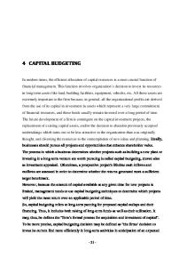
Stages of Capital Budgeting Capital budgeting is the process of making long-run planning decisions for investments in projects. In much of accounting, income is calculated on a period-by-period basis. In choosing investments, however, managers make a selection from among a group of multiple projects, each of which may span several periods. Exhibit 21-1 illustrates these two different, yet intersecting, dimensions of cost analysis: (1) horizontally across, as the project dimension, and (2) vertically upward, as the accounting-period dimension. Each project is represented as a horizontal rectangle starting and ending at different times and stretching over time spans longer than one year. The vertical rectangle for the 2012 accounting period, for example, represents the dimensions of income determination and routine annual planning and control that cuts across all projects that are ongoing that year. Capital budgeting analyzes each project by considering all the lifespan cash flows from its initial investment through its termination and is analogous to life-cycle budgeting and costing (Chapter 12, pp. 451–453). For example, when Honda considers a new line of automobiles, it begins by estimating all potential revenues from the new line as well as any costs that will be incurred along its life cycle, which may be as long as 10 years. Only after examining the potential costs and benefits across all of the business functions in the value chain, from research and development (R&D) to customer service, across the entire lifespan of the new-car project, does Honda decide whether the new model is a wise investment. Capital budgeting is both a decision-making and a control tool. Like the five-step decision process that we have emphasized throughout this book, there are five stages to the capital budgeting process: Stage 1: Identify Projects Identify potential capital investments that agree with the organization’s strategy. For example, when the Microsoft Office group sought a strategy of product differentiation, it listed possible upgrades and changes from its present offering. Alternatively, a strategy of cost leadership could be promoted by projects that improve productivity and efficiency. In the case of a manufacturer of computer hardware such as Dell, this includes the outsourcing of certain components to lower-cost contract

Learning Objective

1

Understand the five stages of capital budgeting for a project . . . identify projects; obtain information; make predictions; make decisions; and implement the decision, evaluate performance, and learn

740 䊉 CHAPTER 21 CAPITAL BUDGETING AND COST ANALYSIS

Exhibit 21-1

Project M

The Project and Time Dimensions of Capital Budgeting

Project N Project O Project P 2010

2011

2013 2012 Accounting Period

2014

2015

manufacturing facilities located overseas. Identifying which types of capital projects to invest in is largely the responsibility of senior line managers. Stage 2: Obtain Information Gather information from all parts of the value chain to evaluate alternative projects. Returning to the new car example at Honda, in this stage, marketing is queried for potential revenue numbers, plant managers are asked about assembly times, and suppliers are consulted about prices and the availability of key components. Some projects may even be rejected at this stage. For example, suppose Honda learns that the car simply cannot be built using existing plants. It may then opt to cancel the project altogether. Stage 3: Make Predictions Forecast all potential cash flows attributable to the alternative projects. Capital investment projects generally involve substantial initial outlays, which are recouped over time through annual cash inflows and the disposal values from the termination of the project. As a result, they require the firm to make forecasts of cash flows several years into the future. BMW, for example, estimates yearly cash flows and sets its investment budgets accordingly using a 12-year planning horizon. Because of the greater uncertainty associated with these predictions, firms typically analyze a wide range of alternate scenarios. In the case of BMW, the marketing group is asked to estimate a band of possible sales figures within a 90% confidence interval. Stage 4: Make Decisions by Choosing Among Alternatives Determine which investment yields the greatest benefit and the least cost to the organization. Using the quantitative information obtained in stage 3, the firm uses any one of several capital budgeting methodologies to determine which project best meets organizational goals. While capital budgeting calculations are typically limited to financial information, managers use their judgment and intuition to factor in qualitative information and strategic considerations as well. For example, even if a proposed new line of cars meets its financial targets on a standalone basis, Honda might decide not to pursue it further if it feels that the new model will lessen Honda’s perceived quality among consumers and affect the value of the firm’s brand. Stage 5: Implement the Decision, Evaluate Performance, and Learn Given the complexities of capital investment decisions and the long time horizons they span, this stage can be separated into two phases: 䊏

Obtain funding and make the investments selected in stage 4. Sources of funding include internally generated cash flow as well as equity and debt securities sold in capital markets. Making capital investments is often an arduous task, laden with the purchase of many different goods and services. If Honda opts to build a new car, it must order steel, aluminum, paint, and so on. If some of the planned supplies are unavailable, managers must revisit and determine the economic feasibility of substituting the missing material with alternative inputs.

䊏

Track realized cash flows, compare against estimated numbers, and revise plans if necessary. As the cash outflows and inflows begin to accumulate, managers can verify whether the predictions made in stage 3 agree with the actual flows of cash from the project. When the BMW group initially released the new Mini, its realized sales were substantially higher than the original demand estimates. BMW responded by manufacturing more cars to meet the higher demand. It also decided to expand the Mini line to include convertibles and the larger Clubman model.

DISCOUNTED CASH FLOW 䊉 741

To illustrate capital budgeting, consider Top-Spin tennis racquets. Top-Spin was one of the first major tennis-racquet producers to introduce graphite in its racquets. This allowed Top-Spin to produce some of the lightest and stiffest racquets in the market. However, new carbon-fiber impregnated racquets are even lighter and stiffer than their graphite counterparts. Top-Spin has always been an innovator in the tennis-racquet industry, and wants to stay that way, so in stage 1, it identifies the carbon fiber racquet project. In the information gathering stage (stage 2), the company learns that it could feasibly begin using carbon-fiber in its racquets as early as 2011 if it replaces one of its graphite forming machines with a carbon-fiber weaving machine. After collecting additional data, Top-Spin begins to forecast future cash flows if it invests in the new machine (stage 3). Top-Spin estimates that it can purchase a carbon-fiber weaving machine with a useful life of five years for a net after-tax initial investment of $379,100, which is calculated as follows: Cost of new machine Investment in working capital Cash flow from disposing of existing machine (after-tax) Net initial investment for new machine

$390,000 9,000 ƒƒ(19,900) $379,100

Working capital refers to the difference between current assets and current liabilities. New projects often necessitate additional investments in current assets such as inventories and receivables. In the case of Top-Spin, the purchase of the new machine is accompanied by an outlay of $9,000 for supplies and spare parts inventory. At the end of the project, the $9,000 in supplies and spare parts inventory is liquidated, resulting in a cash inflow. However, the machine itself is believed to have no terminal disposal value after five years. Managers estimate that by introducing carbon-fiber impregnated racquets, operating cash inflows (cash revenues minus cash operating costs) will increase by $100,000 (after tax) in the first four years and $91,000 in year 5. To simplify the analysis, suppose that all cash flows occur at the end of each year. Note that cash flow at the end of the fifth year also increases by $100,000, $91,000 in operating cash inflows and $9,000 in working capital. Management next calculates the costs and benefits of the proposed project (stage 4). This chapter discusses four capital budgeting methods to analyze financial information: 1. 2. 3. 4.

Decision Point What are the five stages of capital budgeting?

Net present value (NPV) Internal rate of return (IRR) Payback Accrual accounting rate of return (AARR)

Both the net present value (NPV) and internal rate of return (IRR) methods use discounted cash flows, which we discuss in the following section.

Discounted Cash Flow Discounted cash flow (DCF) methods measure all expected future cash inflows and outflows of a project discounted back to the present point in time. The key feature of DCF methods is the time value of money, which means that a dollar (or any other monetary unit) received today is worth more than a dollar received at any future time. The reason is that $1 received today can be invested at, say, 10% per year so that it grows to $1.10 at the end of one year. The time value of money is the opportunity cost (the return of $0.10 forgone per year) from not having the money today. In this example, $1 received one year from now is worth $1 , 1.10 = $0.9091 today. Similarly, $100 received one year from now will be weighted by 0.9091 to yield a discounted cash flow of $90.91, which is today’s value of that $100 next year. In this way, discounted cash flow methods explicitly weigh cash flows by the time value of money. Note that DCF focuses exclusively on cash inflows and outflows rather than on operating income as determined by accrual accounting. The compound interest tables and formulas used in DCF analysis are in Appendix A, pages 839–845. If you are unfamiliar with compound interest, do not proceed until you have studied Appendix A, as the tables in Appendix A will be used frequently in this chapter.

Learning Objective

2

Use and evaluate the two main discounted cash flow (DCF) methods: the net present value (NPV) method and the internal rate-of-return (IRR) method . . . to explicitly consider all project cash flows and the time value of money

742 䊉 CHAPTER 21 CAPITAL BUDGETING AND COST ANALYSIS

The two DCF methods we describe are the net present value (NPV) method and the internal rate-of-return (IRR) method. Both DCF methods use what is called the required rate of return (RRR), the minimum acceptable annual rate of return on an investment. The RRR is internally set, usually by upper management, and typically reflects the return that an organization could expect to receive elsewhere for an investment of comparable risk. The RRR is also called the discount rate, hurdle rate, cost of capital, or opportunity cost of capital. Suppose the CFO at Top-Spin has set the required rate of return for the firm’s investments at 8% per year.

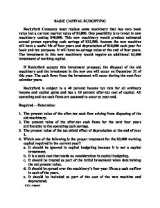
Net Present Value Method The net present value (NPV) method calculates the expected monetary gain or loss from a project by discounting all expected future cash inflows and outflows back to the present point in time using the required rate of return. To use the NPV method, apply the following three steps: Step 1: Draw a Sketch of Relevant Cash Inflows and Outflows. The right side of Exhibit 21-2 shows arrows that depict the cash flows of the new carbon-fiber machine. The sketch helps the decision maker visualize and organize the data in a systematic way. Note that parentheses denote relevant cash outflows throughout all exhibits in Chapter 21. Exhibit 21-2 includes the outflow for the acquisition of the new machine at the start of year 1 (also referred to as end of year 0), and the inflows over the subsequent five years. The NPV method specifies cash flows regardless of the source of the cash flows, such as from operations, purchase or sale of equipment, or investment in or recovery of working capital. However, accrual-accounting concepts such as sales made on credit or noncash expenses are not included since the focus is on cash inflows and outflows.

Exhibit 21-2

Net Present Value Method: Top-Spin’s Carbon-Fiber Machine

A

B

C

Net initial investment Useful life Annual cash inflow Required rate of return

1 2 3 4

D

E

F

G

H

I

$ 379,100 5 years $ 100,000 8%

5

Present Value of Cash Flow

6 7

Present Value of $1 Discounted at 8%

14 15

NPV if new machine purchased

$ 20,200

Approach 2: Using Annuity Tableb 18 Net initial investment

$ (379,100)

9 10 11 12 13

Sketch of Relevant Cash Flows at End of Each Year 1 2 3 4

5

a

Approach 1: Discounting Each Year’s Cash Flow Separately $(379,100) Net initial investment 92,600 85,700 Annual cash inflow 79,400 73,500 68,100

8

0

1.000 0.926 0.857 0.794 0.735 0.681

$(379,100)

1.000

$(379,100)

$100,000 $100,000 $100,000 $100,000 $100,000

16 17

$1 0 0 ,0 0 0

19

$100,000

$100,000

$100,000

$100,000

20 21

Annual cash inflow

22 NPV if new machine purchased

399,300

3.993

$ 20,200

23 24 25 26

Note: Parentheses denote relevant cash outflows throughout all exhibits in Chapter 21. 2 a Present values from Table 2, Appendix A at the end of the book. For example, 0.857 = 1 ÷ (1.08) . b

Annuity present value from Table 4, Appendix A. The annuity value of 3.993 is the sum of the individual discount rates 0.926 + 0.857 + 0.794 + 0.735 + 0.681.

DISCOUNTED CASH FLOW 䊉 743

Step 2: Discount the Cash Flows Using the Correct Compound Interest Table from Appendix A and Sum Them. In the Top-Spin example, we can discount each year’s cash flow separately using Table 2, or we can compute the present value of an annuity, a series of equal cash flows at equal time intervals, using Table 4. (Both tables are in Appendix A.) If we use Table 2, we find the discount factors for periods 1–5 under the 8% column. Approach 1 in Exhibit 21-2 uses the five discount factors. To obtain the present value amount, multiply each discount factor by the corresponding amount represented by the arrow on the right in Exhibit 21-2 ( - $379,100 * 1.000; $100,000 * 0.926; and so on to $100,000 * 0.681). Because the investment in the new machine produces an annuity, we may also use Table 4. Under Approach 2, we find that the annuity factor for five periods under the 8% column is 3.993, which is the sum of the five discount factors used in Approach 1. We multiply the uniform annual cash inflow by this factor to obtain the present value of the inflows ($399,300 = $100,000 * 3.993). Subtracting the initial investment then reveals the NPV of the project as $20,200 ($20,200 = $399,300 - $379,100). Step 3: Make the Project Decision on the Basis of the Calculated NPV. If NPV is zero or positive, financial considerations suggest that the project should be accepted; its expected rate of return equals or exceeds the required rate of return. If NPV is negative, the project should be rejected; its expected rate of return is below the required rate of return. Exhibit 21-2 calculates an NPV of $20,200 at the required rate of return of 8% per year. The project is acceptable based on financial information. The cash flows from the project are adequate (1) to recover the net initial investment in the project and (2) to earn a return greater than 8% per year on the investment tied up in the project over its useful life. Managers must also weigh nonfinancial factors such as the effect that purchasing the machine will have on Top-Spin’s brand. This is a nonfinancial factor because the financial benefits that accrue from Top-Spin’s brand are very difficult to estimate. Nevertheless, managers must consider brand effects before reaching a final decision. Suppose, for example, that the NPV of the carbon-fiber machine is negative. Management may still decide to buy the machine if it maintains Top-Spin’s technological image and helps sell other Top-Spin products. Pause here. Do not proceed until you understand what you see in Exhibit 21-2. Compare Approach 1 with Approach 2 in Exhibit 21-2 to see how Table 4 in Appendix A merely aggregates the present value factors of Table 2. That is, the fundamental table is Table 2. Table 4 simply reduces calculations when there is an annuity.

Internal Rate-of-Return Method The internal rate-of-return (IRR) method calculates the discount rate at which an investment’s present value of all expected cash inflows equals the present value of its expected cash outflows. That is, the IRR is the discount rate that makes NPV = $0. Exhibit 21-3 presents the cash flows and shows the calculation of NPV using a 10% annual discount rate for Top-Spin’s carbon-fiber project. At a 10% discount rate, the NPV of the project is $0. Therefore, IRR is 10% per year. How do managers determine the discount rate that yields NPV = $0? In most cases, managers or analysts solving capital budgeting problems use a calculator or computer program to provide the internal rate of return. The following trial-and-error approach can also provide the answer. Step 1: Use a discount rate and calculate the project’s NPV. Step 2: If the calculated NPV is less than zero, use a lower discount rate. (A lower discount rate will increase NPV. Remember that we are trying to find a discount rate for which NPV = $0.) If NPV is greater than zero, use a higher discount rate to lower NPV. Keep adjusting the discount rate until NPV = $0. In the Top-Spin example, a discount rate of 8% yields an NPV of + $20,200 (see Exhibit 21-2). A discount rate of 12% yields an NPV of - $18,600 (3.605, the present value annuity factor from Table 4, * $100,000 minus $379,100). Therefore, the discount rate that makes NPV = $0 must lie between 8% and 12%. We use 10% and get NPV = $0. Hence, the IRR is 10% per year.

744 䊉 CHAPTER 21 CAPITAL BUDGETING AND COST ANALYSIS

Exhibit 21-3

Internal Rate-of-Return Method: Top-Spin’s Carbon-Fiber Machinea

A

B

C

D

Net initial investment Useful life Annual cash inflow Annual discount rate

1 2 3 4

E

F

G

H

I

$ 379,100 5 years $ 100,000 10%

5

Present Value Present Value of of Cash Flow $1 Discounted at 10%

6 7 8 9 10 11 12 13 14

0

Sketch of Relevant Cash Flows at End of Each Year 1 2 3 4

5

b

Approach 1: Discounting Each Year’s Cash Flow Separately $(379,100) Net initial investment 90,900 82,600 Annual cash inflow 75,100 68,300 62,100

c 15 NPV if new machine purchased (the zero difference proves that 16

$

1.000 0.909 0.826 0.751 0.683 0.621

$(379,100)

1.000

$(379,100)

$100,000 $100,000 $100,000 $100,000 $100,000

0

the internal rate of return is 10%)

17 18 19 20 21

Approach 2: Using Annuity Table Net initial investment

$ (379,100)

$1 0 0 ,0 0 0

22

Annual cash inflow 24 NPV if new machine purchased 23

379,100 $ 0

$100,000

$100,000

$100,000

$100,000

3.791d

25 26 27 28 29 30 31

Note: Parentheses denote relevant cash outflows throughout all exhibits in Chapter 21. The internal rate of return is computed by methods explained on pp. 743–744. b Present values from Table 2, Appendix A at the end of the book. c Sum is $(100) due to rounding. We round to $0. d Annuity present value from Table 4, Appendix A. The annuity table value of 3.791 is the sum of the individual discount rates 0.909 + 0.826 + 0.751 + 0.683 + 0.621, subject to rounding. a

The step-by-step computations of internal rate of return are easier when the cash inflows are constant, as in our Top-Spin example. Information from Exhibit 21-3 can be expressed as follows: $379,100 = Present value of annuity of $100,000 at X% per year for five years

Or, what factor F in Table 4 (in Appendix A) will satisfy this equation? $379,100 = $100,000F F = $379,100 , $100,000 = 3.791

On the five-period line of Table 4, find the percentage column that is closest to 3.791. It is exactly 10%. If the factor (F) falls between the factors in two columns, straight-line interpolation is used to approximate IRR. This interpolation is illustrated in the Problem for Self-Study (pp. 759–760). A project is accepted only if IRR equals or exceeds required rate of return (RRR). In the Top-Spin example, the carbon-fiber machine has an IRR of 10%, which is greater than the RRR of 8%. On the basis of financial factors, Top-Spin should invest in the new machine. In general, the NPV and IRR decision rules result in consistent project acceptance or rejection decisions. If IRR exceeds RRR, then the project has a positive NPV (favoring acceptance). If IRR equals RRR, NPV = $0, so project acceptance and rejection yield the same value. If IRR is less than RRR, NPV is negative (favoring rejection). Obviously, managers prefer projects with higher IRRs to projects with lower IRRs, if all

DISCOUNTED CASH FLOW 䊉 745

other things are equal. The IRR of 10% means the cash inflows from the project are adequate to (1) recover the net initial investment in the project and (2) earn a return of exactly 10% on the investment tied up in the project over its useful life.

Comparison of Net Present Value and Internal Rate-of-Return Methods The NPV method is generally regarded as the preferred method for project selection decisions. The reason is that choosing projects using the NPV criterion leads to shareholder value maximization. At an intuitive level, this occurs because the NPV measure for a project captures the value, in today’s dollars, of the surplus the project generates for the firm’s shareholders, over and above the required rate of return.2 Next, we highlight some of the limitations of the IRR method relative to the NPV technique. One advantage of the NPV method is that it expresses computations in dollars, not in percentages. Therefore, we can sum NPVs of individual projects to calculate an NPV of a combination or portfolio of projects. In contrast, IRRs of individual projects cannot be added or averaged to represent the IRR of a combination of projects. A second advantage is that the NPV of a project can always be computed and expressed as a unique number. From the sign and magnitude of this number, the firm can then make an accurate assessment of the financial consequences of accepting or rejecting the project. Under the IRR method, it is possible that more than one IRR may exist for a given project. In other words, there may be multiple discount rates that equate the NPV of a set of cash flows to zero. This is especially true when the signs of the cash flows switch over time; that is, when there are outflows, followed by inflows, followed by additional outflows and so forth. In such cases, it is difficult to know which of the IRR estimates should be compared to the firm’s required rate of return. A third advantage of the NPV method is that it can be used when the RRR varies over the life of a project. Suppose Top-Spin’s management sets an RRR of 9% per year in years 1 and 2 and 12% per year in years 3, 4, and 5. Total present value of the cash inflows can be calculated as $378,100 (computations not shown). It is not possible to use the IRR method in this case. That’s because different RRRs in different years mean there is no single RRR that the IRR (a single figure) can be compared against to decide if the project should be accepted or rejected. Finally, there are specific settings in which the IRR method is prone to indicating erroneous decisions, such as when comparing mutually exclusive projects with unequal lives or unequal levels of initial investment. The reason is that the IRR method implicitly assumes that project cash flows can be reinvested at the project’s rate of return. The NPV method, in contrast, accurately assumes that project cash flows can only be reinvested at the company’s required rate of return. Despite its limitations, surveys report widespread use of the IRR method.3 Why? Probably because managers find the percentage return computed under the IRR method easy to understand and compare. Moreover, in most instances where a single project is being evaluated, their decisions would likely be unaffected by using IRR or NPV.

Sensitivity Analysis To present the basics of the NPV and IRR methods, we have assumed that the expected values of cash flows will occur for certain. In reality, there is substantial uncertainty associated with the prediction of future cash flows. To examine how a result will change if the predicted financial outcomes are not achieved or if an underlying assumption changes, managers use sensitivity analysis, a “what-if” technique introduced in Chapter 3. A common way to apply sensitivity analysis in capital budgeting decisions is to vary each of the inputs to the NPV calculation by a certain percentage and assess the effect of the change on the project’s NPV. Sensitivity analysis can take on other forms as well. Suppose the manager at Top-Spin believes forecasted cash flows are difficult to predict. 2 3

More detailed explanations of the preeminence of the NPV criterion can be found in corporate finance texts. In a recent survey, John Graham and Campbell Harvey found that 75.7% of CFOs always or almost always used IRR for capital budgeting decisions, while a slightly smaller number, 74.9%, always or almost always used the NPV criterion.

746 䊉 CHAPTER 21 CAPITAL BUDGETING AND COST ANALYSIS

Exhibit 21-4 Net Present Value Calculations for TopSpin’s Carbon-Fiber Machine Under Different Assumptions of Annual Cash Flows and Required Rates of Returna

A 1

Required Rate of Return 6% 8% 10%

2 3 4 5 6 7

a

B

C

$ 80,000 $(42,140) $(59,660) $(75,820)

D

E

Annual Cash Flows $ 90,000 $100,000 $110,000 $ (20) $ 42,100 $ 84,220 $(19,730) $ 20,200 $ 60,130 $(37,910) $ 0 $ 37,910

F

$120,000 $126,340 $100,060 $ 75,820

All calculated amounts assume the project’s useful life is five years.

She asks, “What are the minimum annual cash inflows that make the investment in a new carbon-fiber machine acceptable—that is, what inflows lead to an NPV = $0?” For the data in Exhibit 21-2, let A = Annual cash flow and let NPV = $0. Net initial investment is $379,100, and the present value factor at the 8% required annual rate of return for a five-year annuity of $1 is 3.993. Then, NPV = $0 3.993A - $379,100 = $0 3.993A = $379,100 A = $94,941

Decision Point What are the two primary discounted cash flow (DCF) methods for project evaluation?

At the discount rate of 8% per year, the annual (after tax) cash inflows can decrease to $94,941 (a decline of $100,000 - $94,941 = $5,059) before the NPV falls to $0. If the manager believes she can attain annual cash inflows of at least $94,941, she can justify investing in the carbon-fiber machine on financial grounds. Exhibit 21-4 shows that variations in the annual cash inflows or RRR significantly affect the NPV of the carbon-fiber machine project. NPVs can also vary with different useful lives of a project. Sensitivity analysis helps managers to focus on decisions that are most sensitive to different assumptions and to worry less about decisions that are not so sensitive.

Payback Method Learning Objective

3

Use and evaluate the payback and discounted payback methods . . . to calculate the time it takes to recoup the investment

We now consider the third method for analyzing the financial aspects of projects. The payback method measures the time it will take to recoup, in the form of expected future cash flows, the net initial investment in a project. As in NPV and IRR, payback does not distinguish among the sources of cash flows, such as from operations, purchase or sale of equipment, or investment or recovery of working capital. Payback is simpler to calculate when a project has uniform cash flows, as opposed to nonuniform cash flows. We consider the former case first.

Uniform Cash Flows In the Top-Spin example, the carbon-fiber machine costs $379,100, has a five-year expected useful life, and generates $100,000 uniform cash flow each year. Calculation of the payback period is as follows: Payback period = =

4

Net initial investment Uniform increase in annual future cash flows $379,100 = 3.8 years4 $100,000

Cash inflows from the new carbon-fiber machine occur uniformly throughout the year, but for simplicity in calculating NPV and IRR, we assume they occur at the end of each year. A literal interpretation of this assumption would imply a payback of four years because Top-Spin will only recover its investment when cash inflows occur at the end of year 4. The calculations shown in the chapter, however, better approximate Top-Spin’s payback on the basis of uniform cash flows throughout the year.

PAYBACK METHOD 䊉 747

The payback method highlights liquidity, a factor that often plays a role in capital budgeting decisions, particularly when the investments are large. Managers prefer projects with shorter payback periods (projects that are more liquid) to projects with longer payback periods, if all other things are equal. Projects with shorter payback periods give an organization more flexibility because funds for other projects become available sooner. Also, managers are less confident about cash flow predictions that stretch far into the future, again favoring shorter payback periods. Unlike the NPV and IRR methods where management selected a RRR, under the payback method, management chooses a cutoff period for a project. Projects with a payback period that is less than the cutoff period are considered acceptable, and those with a payback period that is longer than the cutoff period are rejected. Japanese companies favor the payback method over other methods and use cutoff periods ranging from three to five years depending on the risks involved with the project. In general, modern risk management calls for using shorter cutoff periods for riskier projects. If Top-Spin’s cutoff period under the payback method is three years, it will reject the new machine. The payback method is easy to understand. As in DCF methods, the payback method is not affected by accrual accounting conventions such as depreciation. Payback is a useful measure when (1) preliminary screening of many proposals is necessary, (2) interest rates are high, and (3) the expected cash flows in later years of a project are highly uncertain. Under these conditions, companies give much more weight to cash flows in early periods of a capital budgeting project and to recovering the investments they have made, thereby making the payback criterion especially relevant. Two weaknesses of the payback method are that (1) it fails to explicitly incorporate the time value of money and (2) it does not consider a project’s cash flows after the payback period. Consider an alternative to the $379,100 carbon-fiber machine. Another carbon-fiber machine, with a three-year useful life and no terminal disposal value, requires only a $300,000 net initial investment and will also result in cash inflows of $100,000 per year. First, compare the payback periods: Machine 1 =

$379,100 = 3.8 years $100,000

Machine 2 =

$300,000 = 3.0 years $100,000

The payback criterion favors machine 2, with the shorter payback. If the cutoff period were three years, machine 1 would fail to meet the payback criterion. Consider next the NPV of the two investment options using Top-Spin’s 8% required rate of return for the carbon-fiber machine investment. At a discount rate of 8%, the NPV of machine 2 is - $42,300 (2.577, the present value annuity factor for three years at 8% per year from Table 4, times $100,000 = $257,700 minus net initial investment of $300,000). Machine 1, as we know, has a positive NPV of $20,200 (from Exhibit 21-2). The NPV criterion suggests Top-Spin should acquire machine 1. Machine 2, with a negative NPV, would fail to meet the NPV criterion. The payback method gives a different answer from the NPV method in this example because the payback method ignores cash flows after the payback period and ignores the time value of money. Another problem with the payback method is that choosing too short a cutoff period for project acceptance may promote the selection of only short-lived projects. An organization will tend to reject long-run, positive-NPV projects. Despite these differences, companies find it useful to look at both NPV and payback when making capital investment decisions.

Nonuniform Cash Flows When cash flows are not uniform, the payback computation takes a cumulative form: The cash flows over successive years are accumulated until the amount of net initial investment is recovered. Assume that Venture Law Group is considering the purchase of videoconferencing equipment for $150,000. The equipment is expected to provide a total cash savings of $340,000 over the next five years, due to reduced travel costs and

748 䊉 CHAPTER 21 CAPITAL BUDGETING AND COST ANALYSIS

more effective use of associates’ time. The cash savings occur uniformly throughout each year, but are not uniform across years.

Year 0 1 2 3 4 5

Cash Savings — $50,000 55,000 60,000 85,000 90,000

Cumulative Cash Savings — $ 50,000 105,000 165,000 250,000 340,000

Net Initial Investment Unrecovered at End of Year $150,000 100,000 45,000 — — —

It is clear from the chart that payback occurs during the third year. Straight-line interpolation within the third year reveals that the final $45,000 needed to recover the $150,000 investment (that is, $150,000 - $105,000 recovered by the end of year 2) will be achieved threequarters of the way through year 3 (in which $60,000 of cash savings occur): Payback period = 2 years + a

$45,000 * 1 yearb = 2.75 years $60,000

It is relatively simple to adjust the payback method to incorporate the time value of money by using a similar cumulative approach. The discounted payback method calculates the amount of time required for the discounted expected future cash flows to recoup the net initial investment in a project. For the videoconferencing example, we can modify the preceding chart by discounting the cash flows at the 8% required rate of return.

Year (1) 0 1 2 3 4 5

Cash Savings (2) — $50,000 55,000 60,000 85,000 90,000

Present Value of $1 Discounted at 8% (3) 1.000 0.926 0.857 0.794 0.735 0.681

Discounted Cash Savings (4) = (2)  (3) — $46,300 47,135 47,640 62,475 61,290

Cumulative Discounted Cash Savings (5) — $ 46,300 93,435 141,075 203,550 264,840

Net Initial Investment Unrecovered at End of Year (6) $150,000 103,700 56,565 8,925 — —

The fourth column represents the present values of the future cash savings. It is evident from the chart that discounted payback occurs between years 3 and 4. At the end of the third year, $8,925 of the initial investment is still unrecovered. Comparing this to the $62,475 in present value of savings achieved in the fourth year, straight-line interpolation then reveals that the discounted payback period is exactly one-seventh of the way into the fourth year: Discounted payback period = 3 years + a

Decision Point What are the payback and discounted payback methods? What are their main weaknesses?

$8,925 * 1 yearb = 3.14 years $62,475

While discounted payback does incorporate the time value of money, it is still subject to the other criticism of the payback method—cash flows beyond the discounted payback period are ignored, resulting in a bias toward shorter-term projects. Companies such as Hewlett-Packard value the discounted payback method (HP refers to it as “breakeven time”) because they view longer-term cash flows as inherently unpredictable in highgrowth industries. Finally, the videoconferencing example has a single cash outflow of $150,000 in year 0. When a project has multiple cash outflows occurring at different points in time, these outflows are first aggregated to obtain a total cash-outflow figure for the project. For computing the payback period, the cash flows are simply added, with no adjustment for the time value of money. For calculating the discounted payback period, the present values of the outflows are added instead.

ACCRUAL ACCOUNTING RATE-OF-RETURN METHOD 䊉 749

Accrual Accounting Rate-of-Return Method We now consider a fourth method for analyzing the financial aspects of capital budgeting projects. The accrual accounting rate of return (AARR) method divides the average annual (accrual accounting) income of a project by a measure of the investment in it. We illustrate AARR for the Top-Spin example using the project’s net initial investment as the amount in the denominator: Increase in expected average annual after-tax operating income Accrual accounting = Net initial investment rate of return

If Top-Spin purchases the new carbon-fiber machine, its net initial investment is $379,100. The increase in expected average annual after-tax operating cash inflows is $98,200. This amount is the expected after-tax total operating cash inflows of $491,000 ($100,000 for four years and $91,000 in year 5), divided by the time horizon of five years. Suppose that the new machine results in additional depreciation deductions of $70,000 per year ($78,000 in annual depreciation for the new machine, relative to $8,000 per year on the existing machine).5 The increase in expected average annual after-tax income is therefore $28,200 (the difference between the cash flow increase of $98,200 and the depreciation increase of $70,000). The AARR on net initial investment is computed as follows: AARR =

$28,200 per year $98,200 - $70,000 = = 0.074, or 7.4% per year $379,100 $379,100

The 7.4% figure for AARR indicates the average rate at which a dollar of investment generates after-tax operating income. The new carbon-fiber machine has a low AARR for two reasons: (1) the use of net initial investment as the denominator, and (2) the use of income as the numerator, which necessitates deducting depreciation charges from the annual operating cash flows. To mitigate the first issue, many companies calculate AARR using an average level of investment. This alternative procedure recognizes that the book value of the investment declines over time. In its simplest form, average investment for Top-Spin is calculated as the arithmetic mean of the net initial investment of $379,100 and the net terminal cash flow of $9,000 (terminal disposal value of machine of $0, plus the terminal recovery of working capital of $9,000): Average investment Net initial investment + Net terminal cash flow = over five years 2 $379,100 + $9,000 = = $194,050 2

The AARR on average investment is then calculated as follows: AARR =

$28,200 = 0.145, or 14.5% per year $194,050

Our point here is that companies vary in how they calculate AARR. There is no uniformly preferred approach. Be sure you understand how AARR is defined in each individual situation. Projects whose AARR exceeds a specified hurdle required rate of return are regarded as acceptable (the higher the AARR, the better the project is considered to be). The AARR method is similar to the IRR method in that both methods calculate a rate-of-return percentage. The AARR method calculates return using operating-income numbers after considering accruals and taxes, whereas the IRR method calculates return on the basis of after-tax cash flows and the time value of money. Because cash flows and time value of money are central to capital budgeting decisions, the IRR method is regarded as better than the AARR method. AARR computations are easy to understand, and they use numbers reported in the financial statements. AARR gives managers an idea of how the accounting numbers they will report in the future will be affected if a project is accepted. Unlike the payback method, 5

We provide further details on these numbers in the next section; see p. 750.

Learning Objective

4

Use and evaluate the accrual accounting rate-of-return (AARR) method . . . after-tax operating income divided by investment

750 䊉 CHAPTER 21 CAPITAL BUDGETING AND COST ANALYSIS

Decision Point What are the strengths and weaknesses of the accrual accounting rate-of-return (AARR) method for evaluating long-term projects?

which ignores cash flows after the payback period, the AARR method considers income earned throughout a project’s expected useful life. Unlike the NPV method, the AARR method uses accrual accounting income numbers, it does not track cash flows, and it ignores the time value of money. Critics cite these arguments as drawbacks of the AARR method. Overall, keep in mind that companies frequently use multiple methods for evaluating capital investment decisions. When different methods lead to different rankings of projects, finance theory suggests that more weight be given to the NPV method because the assumptions made by the NPV method are most consistent with making decisions that maximize company value.

Relevant Cash Flows in Discounted Cash Flow Analysis Learning Objective

5

Identify relevant cash inflows and outflows for capital budgeting decisions . . . the differences in expected future cash flows resulting from the investment

So far, we have examined methods for evaluating long-term projects in settings where the expected future cash flows of interest were assumed to be known. One of the biggest challenges in capital budgeting, particularly DCF analysis, however, is determining which cash flows are relevant in making an investment selection. Relevant cash flows are the differences in expected future cash flows as a result of making the investment. In the Top-Spin example, the relevant cash flows are the differences in expected future cash flows between continuing to use the old technology and updating its technology with the purchase of a new machine. When reading this section, focus on identifying expected future cash flows and the differences in expected future cash flows. To illustrate relevant cash flow analysis, consider a more complex version of the Top-Spin example with these additional assumptions: 䊏

䊏

䊏

䊏

䊏

䊏

Top-Spin is a profitable company. The income tax rate is 40% of operating income each year. The before-tax additional operating cash inflows from the carbon-fiber machine are $120,000 in years 1 through 4 and $105,000 in year 5. For tax purposes, Top-Spin uses the straight-line depreciation method and assumes no terminal disposal value. Gains or losses on the sale of depreciable assets are taxed at the same rate as ordinary income. The tax effects of cash inflows and outflows occur at the same time that the cash inflows and outflows occur. Top-Spin uses an 8% required rate of return for discounting after-tax cash flows.

Summary data for the machines follow:

Purchase price Current book value Current disposal value Terminal disposal value five years from now Annual depreciation Working capital required a$40,000 b$390,000

Old Graphite Machine — $40,000 6,500 0 8,000a 6,000

New Carbon-Fiber Machine $390,000 — Not applicable 0 78,000b 15,000

, 5 years = $8,000 annual depreciation. , 5 years = $78,000 annual depreciation.

Relevant After-Tax Flows We use the concepts of differential cost and differential revenue introduced in Chapter 11. We compare (1) the after-tax cash outflows as a result of replacing the old machine with (2) the additional after-tax cash inflows generated from using the new machine rather than the old machine. As Benjamin Franklin said, “Two things in life are certain: death and taxes.” Income taxes are a fact of life for most corporations and individuals. It is important first to

RELEVANT CASH FLOWS IN DISCOUNTED CASH FLOW ANALYSIS 䊉 751

understand how income taxes affect cash flows in each year. Exhibit 21-5 shows how investing in the new machine will affect Top-Spin’s cash flow from operations and its income taxes in year 1. Recall that Top-Spin will generate $120,000 in before-tax additional operating cash inflows by investing in the new machine (p. 750), but it will record additional depreciation of $70,000 ($78,000 - $8,000) for tax purposes. Panel A shows that the year 1 cash flow from operations, net of income taxes, equals $100,000, using two methods based on the income statement. The first method focuses on cash items only, the $120,000 operating cash inflows minus income taxes of $20,000. The second method starts with the $30,000 increase in net income (calculated after subtracting the $70,000 additional depreciation deductions for income tax purposes) and adds back that $70,000, because depreciation is an operating cost that reduces net income but is a noncash item itself. Panel B of Exhibit 21-5 describes a third method that we will use frequently to compute cash flow from operations, net of income taxes. The easiest way to interpret the third method is to think of the government as a 40% (equal to the tax rate) partner in Top-Spin. Each time Top-Spin obtains operating cash inflows, C, its income is higher by C, so it will pay 40% of the operating cash inflows (0.40C) in taxes. This results in additional after-tax cash operating flows of C - 0.40C, which in this example is $120,000 - (0.40 * $120,000) = $72,000, or $120,000 * (1 - 0.40) = $72,000. To achieve the higher operating cash inflows, C, Top-Spin incurs higher depreciation charges, D, from investing in the new machine. Depreciation costs do not directly affect cash flows because depreciation is a noncash cost, but higher depreciation cost lowers Top-Spin’s taxable income by D, saving income tax cash outflows of 0.40D, which in this example is 0.40 * $70,000 = $28,000. Letting t = tax rate, cash flow from operations, net of income taxes, in this example equals the operating cash inflows, C, minus the tax payments on these inflows, t * C, plus the tax savings on depreciation deductions, t * D: $120,000 - (0.40 * $120,000) + (0.40 * $70,000) = $120,000 - $48,000 + $28,000 = $100,000. By the same logic, each time Top-Spin has a gain on the sale of assets, G, it will show tax outflows, t * G; and each time Top-Spin has a loss on the sale of assets, L, it will show tax benefits or savings of t * L.

Exhibit 21-5 PANEL A: Two Methods Based on the Income Statement C D OI T NI

Operating cash inflows from investment in machine Additional depreciation deduction Increase in operating income Income taxes (Income tax rate t  OI ) = 40%  $50,000 Increase in net income Increase in cash flow from operations, net of income taxes Method 1: C  T = $120,000  $20,000 = $100,000 or Method 2: NI + D = $30,000 + $70,000 = $100,000

$120,000 70,000 50,000 20,000 $ 30,000

PANEL B: Item-by-Item Method C t C C  (t  C ) = (1  t )  C D tD (1  t )  C + (t  D ) = C  (t  C ) + (t  D)

Effect of cash operating flows Operating cash inflows from investment in machine Deduct income tax cash outflow at 40% After-tax cash flow from operations (excluding the depreciation effect) Effect of depreciation Additional depreciation deduction, $70,000 Income tax cash savings from additional depreciation deduction at 40%  $70,000 Cash flow from operations, net of income taxes

$120,000 48,000 72,000

28,000 $100,000

Effect on Cash Flow from Operations, Net of Income Taxes, in Year 1 for Top-Spin’s Investment in the New Carbon-Fiber Machine

752 䊉 CHAPTER 21 CAPITAL BUDGETING AND COST ANALYSIS

Categories of Cash Flows A capital investment project typically has three categories of cash flows: (1) net initial investment in the project, which includes the acquisition of assets and any associated additions to working capital, minus the after-tax cash flow from the disposal of existing assets; (2) after-tax cash flow from operations (including income tax cash savings from annual depreciation deductions); and (3) after-tax cash flow from terminal disposal of an asset and recovery of working capital. We use the Top-Spin example to discuss these three categories. As you work through the cash flows in each category, refer to Exhibit 21-6. This exhibit sketches the relevant cash flows for Top-Spin’s decision to purchase the new machine as described in items 1 through 3 here. Note that the total relevant cash flows for each year equal the relevant cash flows used in Exhibits 21-2 and 21-3 to illustrate the NPV and IRR methods. 1. Net Initial Investment. Three components of net-initial-investment cash flows are (a) cash outflow to purchase the machine, (b) cash outflow for working capital, and (c) after-tax cash inflow from current disposal of the old machine. 1a. Initial machine investment. These outflows, made for purchasing plant and equipment, occur at the beginning of the project’s life and include cash outflows for transporting and installing the equipment. In the Top-Spin example, the $390,000 cost (including transportation and installation) of the carbon-fiber machine is an outflow in year 0. These cash flows are relevant to the capital budgeting decision because they will be incurred only if Top-Spin decides to purchase the new machine. 1b. Initial working-capital investment. Initial investments in plant and equipment are usually accompanied by additional investments in working capital. These additional investments take the form of current assets, such as accounts receivable and inventories, minus current liabilities, such as accounts payable. Working-capital investments are similar to plant and equipment investments in that they require cash. The magnitude of the investment generally increases as a function of the level of additional sales generated by the project. However, the exact relationship varies based on the nature of the project and the operating cycle of the industry. Exhibit 21-6

A

Relevant Cash Inflows and Outflows for Top-Spin’s Carbon-Fiber Machine

B

C

1 2 3

1a. 4 1b. 5 1c. 6 7 8 9 10 11 12 13 14 15 16 17 18

Initial machine investment Initial working-capital investment After-tax cash flow from current disposal of old machine Net initial investment 2a. Annual after-tax cash flow from operations (excluding the depreciation effect) 2b. Income tax cash savings from annual depreciation deductions 3a. After-tax cash flow from terminal disposal of machine 3b. After-tax cash flow from recovery of working capital Total relevant cash flows, as shown in Exhibits 21-2 and 21-3

0 $(390,000) (9,000)

D

E

F

G

Sketch of Relevant Cash Flows at End of Year 1 2 3 4

H

5

19,900 (379,100) $ 72,000

$ 72,000

$ 72,000

$ 72,000

$ 63,000

28,000

28,000

28,000

28,000

28,000 0 9,000

$(379,100)

$ 100,000

$100,000

$100,000

$100,000

$100,000

RELEVANT CASH FLOWS IN DISCOUNTED CASH FLOW ANALYSIS 䊉 753

For a given dollar of sales, a maker of heavy equipment, for example, would require more working capital support than Top-Spin, which in turn has to invest more in working capital than a retail grocery store. The Top-Spin example assumes a $9,000 additional investment in working capital (for supplies and spare-parts inventory) if the new machine is acquired. The additional working-capital investment is the difference between working capital required to operate the new machine ($15,000) and working capital required to operate the old machine ($6,000). The $9,000 additional investment in working capital is a cash outflow in year 0 and is returned, that is, becomes a cash inflow, at the end of year 5. 1c. After-tax cash flow from current disposal of old machine. Any cash received from disposal of the old machine is a relevant cash inflow (in year 0). That’s because it is an expected future cash flow that differs between the alternatives of investing and not investing in the new machine. Top-Spin will dispose of the old machine for $6,500 only if it invests in the new carbon-fiber machine. Recall from Chapter 11 (p. 414) that the book value (which is original cost minus accumulated depreciation) of the old equipment is generally irrelevant to the decision since it is a past, or sunk, cost. However, when tax considerations are included, book value does play a role. The reason is that the book value determines the gain or loss on sale of the machine and, therefore, the taxes paid (or saved) on the transaction. Consider the tax consequences of disposing of the old machine. We first have to compute the gain or loss on disposal: Current disposal value of old machine (given, p. 750) Deduct current book value of old machine (given, p. 750) Loss on disposal of machine

$ 6,500 ƒƒ40,000 $(33,500)

Any loss on the sale of assets lowers taxable income and results in tax savings. The after-tax cash flow from disposal of the old machine is as follows: Current disposal value of old machine Tax savings on loss (0.40 * $33,500) After-tax cash inflow from current disposal of old machine

$ 6,500 ƒ13,400 $19,900

The sum of items 1a, 1b, and 1c appears in Exhibit 21-6 as the year 0 net initial investment for the new carbon-fiber machine equal to $379,100 (initial machine investment, $390,000, plus additional working-capital investment, $9,000, minus after-tax cash inflow from current disposal of the old machine, $19,900).6 2. Cash Flow from Operations. This category includes the difference between each year’s cash flow from operations under the two alternatives. Organizations make capital investments to generate future cash inflows. These inflows may result from savings in operating costs, or, as for Top-Spin, from producing and selling additional goods. Annual cash flow from operations can be net outflows in some years. Chevron makes periodic upgrades to its oil extraction equipment, and in years of upgrades, cash flow from operations tends to be negative for the site being upgraded, although in the long-run such upgrades are NPV positive. Always focus on cash flow from operations, not on revenues and expenses under accrual accounting. Top-Spin’s additional operating cash inflows—$120,000 in each of the first four years and $105,000 in the fifth year—are relevant because they are expected future cash flows that will differ between the alternatives of investing and not investing in the new machine. The after-tax effects of these cash flows follow. 2a. Annual after-tax cash flow from operations (excluding the depreciation effect). The 40% tax rate reduces the benefit of the $120,000 additional operating cash

6

To illustrate the case when there is a gain on disposal, suppose that the old machine could be sold now for $50,000 instead. Then, the firm would record a gain on disposal of $10,000 ($50,000 less the book value of $40,000), resulting in additional tax payments of $4,000 (0.40 tax rate  $10,000 gain). The after-tax cash inflow from current disposal would therefore equal $46,000 (the disposal value of $50,000, less the tax payment of $4,000).

754 䊉 CHAPTER 21 CAPITAL BUDGETING AND COST ANALYSIS

inflows for years 1 through 4 with the new carbon-fiber machine. After-tax cash flow (excluding the depreciation effect) is as follows: Annual cash flow from operations with new machine Deduct income tax payments (0.40 * $120,000) Annual after-tax cash flow from operations

$120,000 ƒƒ48,000 $ƒ72,000

For year 5, the after-tax cash flow (excluding the depreciation effect) is as follows: Annual cash flow from operations with new machine Deduct income tax payments (0.40 * $105,000) Annual after-tax cash flow from operations

$105,000 ƒƒ42,000 $ƒ63,000

Exhibit 21-6, item 2a, shows the $72,000 amounts for each of the years 1 through 4 and $63,000 for year 5. To reinforce the idea about focusing on cash flows, consider the following additional fact about the Top-Spin example. Suppose the total plant overhead costs will not change whether the new machine is purchased or the old machine is kept. The production plant’s overhead costs are allocated to individual machines— Top-Spin has several—on the basis of the labor costs for operating each machine. Because the new carbon-fiber machine would have lower labor costs, overhead costs allocated to it would be $30,000 less than the amount allocated to the machine it would replace. How should Top-Spin incorporate the decrease in allocated overhead costs of $30,000 in the relevant cash flow analysis? To answer that question, we need to ask, “Do total overhead costs decrease at Top-Spin’s production plant as a result of acquiring the new machine?” In our example, they do not. Total overhead costs of the production plant remain the same whether or not the new machine is acquired. Only the overhead costs allocated to individual machines change. The overhead costs allocated to the new machine are $30,000 less than the amount allocated to the machine it would replace. This $30,000 difference in overhead would be allocated to other machines in the department. That is, no cash flow savings in total overhead would occur. Therefore, the $30,000 should not be included as part of annual cash savings from operations. Next consider the effects of depreciation. The depreciation line item is itself irrelevant in DCF analysis. That’s because it’s a noncash allocation of costs, whereas DCF is based on inflows and outflows of cash. In DCF methods, the initial cost of equipment is regarded as a lump-sum outflow of cash in year 0. Deducting depreciation expenses from operating cash inflows would result in counting the lump-sum amount twice. However, depreciation results in income tax cash savings. These tax savings are a relevant cash flow. 2b. Income tax cash savings from annual depreciation deductions. Tax deductions for depreciation, in effect, partially offset the cost of acquiring the new carbon-fiber machine. By purchasing the new machine, Top-Spin is able to deduct $78,000 in depreciation each year, relative to the $8,000 depreciation on the old graphite machine. The additional annual depreciation deduction of $70,000 results in incremental income tax cash savings of $70,000  0.4, or $28,000 annually. Exhibit 21-6, item 2b, shows these $28,000 amounts for years 1 through 5.7 For economic-policy reasons, usually to encourage (or in some cases, discourage) investments, tax laws specify which depreciation methods and which depreciable lives are permitted. Suppose the government permitted accelerated depreciation to be used, allowing for higher depreciation deductions in earlier years. If allowable, should Top-Spin use accelerated depreciation? Yes, because there is a general rule in tax planning for profitable companies such as Top-Spin: When there is a legal choice, take the depreciation (or any other deduction) sooner rather than later. Doing so causes the (cash) income tax savings to occur earlier, which increases the project’s NPV. 7

If Top-Spin were a nonprofit foundation not subject to income taxes, cash flow from operations would equal $120,000 in years 1 through 4 and $105,000 in year 5. The revenues would not be reduced by 40%, nor would there be income tax cash savings from the depreciation deduction.

PROJECT MANAGEMENT AND PERFORMANCE EVALUATION 䊉 755

3. Terminal Disposal of Investment. The disposal of the new investment generally increases cash inflow when the project terminates. Errors in forecasting terminal disposal value are seldom critical for long-duration projects, because the present value of amounts to be received in the distant future is usually small. Two components of the terminal disposal value of an investment are (a) after-tax cash flow from terminal disposal of machines and (b) after-tax cash flow from recovery of working capital. 3a. After-tax cash flow from terminal disposal of machines. At the end of the useful life of the project, the machine’s terminal disposal value may be $0 or an amount considerably less than the net initial investment. The relevant cash inflow is the difference in expected after-tax cash inflow from terminal disposal at the end of five years under the two alternatives of purchasing the new machine or keeping the old machine. Although the old machine has a positive terminal disposal value today (year 0), in year 5, it will have a zero terminal value. As such, both the existing and the new machines have zero after-tax cash inflow from terminal disposal in year 5. Hence, the difference in after-tax cash inflow from terminal disposal is also $0. In this example, there are no tax effects at the terminal point because both the existing and new machine have disposal values that equal their book values at the time of disposal (in each case, this value is $0). What if either the existing or the new machine had a terminal value that differed from its book value at the time of disposal? In that case, the approach for computing the terminal inflow is identical to that for calculating the after-tax cash flow from current disposal illustrated earlier in part 1c. 3b. After-tax cash flow from terminal recovery of working-capital investment. The initial investment in working capital is usually fully recouped when the project is terminated. At that time, inventories and accounts receivable necessary to support the project are no longer needed. Top-Spin receives cash equal to the book value of its working capital. Thus, there is no gain or loss on working capital and, hence, no tax consequences. The relevant cash inflow is the difference in the expected working capital recovered under the two alternatives. At the end of year 5, Top-Spin recovers $15,000 cash from working capital if it invests in the new carbon-fiber machine versus $6,000 if it continues to use the old machine. The relevant cash inflow at the end of year 5 if Top-Spin invests in the new machine is thus $9,000 ($15,000 - $6,000). Some capital investment projects reduce working capital. Assume that a computer-integrated manufacturing (CIM) project with a seven-year life will reduce inventories and, hence, working capital by $20 million from, say, $50 million to $30 million. This reduction will be represented as a $20 million cash inflow for the project in year 0. At the end of seven years, the recovery of working capital will show a relevant incremental cash outflow of $20 million. That’s because, at the end of year 7, the company recovers only $30 million of working capital under CIM, rather than the $50 million of working capital it would have recovered had it not implemented CIM. Exhibit 21-6 shows items 3a and 3b in the “year 5” column. The relevant cash flows in Exhibit 21-6 serve as inputs for the four capital budgeting methods described earlier in the chapter.

Project Management and Performance Evaluation We have so far looked at ways to identify relevant cash flows and appropriate techniques for analyzing them. The final stage (stage 5) of capital budgeting begins with implementing the decision, or managing the project.8 This includes management control of the investment activity itself, as well as management control of the project as a whole. Capital budgeting projects, such as purchasing a carbon-fiber machine or videoconferencing equipment, are easier to implement than projects involving building shopping 8

In this section, we do not consider the different options for financing a project (refer to a text on corporate finance for details).

Decision Point What are the relevant cash inflows and outflows for capital budgeting decisions? How should accrual accounting concepts be considered?

Learning Objective

6

Understand issues involved in implementing capital budgeting decisions and evaluating managerial performance . . . the importance of post-investment audits and the correct choice of performance measures

756 䊉 CHAPTER 21 CAPITAL BUDGETING AND COST ANALYSIS

malls or manufacturing plants. The building projects are more complex, so monitoring and controlling the investment schedules and budgets are critical to successfully completing the investment activity. This leads to the second dimension of stage 5 in the capital budgeting process: evaluate performance and learn.

Post-Investment Audits A post-investment audit provides management with feedback about the performance of a project, so management can compare actual results to the costs and benefits expected at the time the project was selected. Suppose actual outcomes (such as additional operating cash flows from the new carbon-fiber machine in the Top-Spin example) are much lower than expected. Management must then investigate to determine if this result occurred because the original estimates were overly optimistic or because of implementation problems. Either of these explanations is a concern. Optimistic estimates may result in the acceptance of a project that should have been rejected. To discourage optimistic estimates, companies such as DuPont maintain records comparing actual results to the estimates made by individual managers when seeking approval for capital investments. Post-investment audits punish inaccurate estimates, and therefore discourage unrealistic forecasts. This prevents managers from overstating project cash inflows and accepting projects that should never have been undertaken. Implementation problems, such as weak project management, poor quality control, or inadequate marketing are also a concern. Post-investment audits help to alert senior management to these problems so that they can be quickly corrected. However, post-investment audits require thoughtfulness and care. They should be done only after project outcomes have stabilized because performing audits too early may yield misleading feedback. Obtaining actual results to compare against estimates is often not easy. For example, additional revenues from the new carbon-fiber technology may not be comparable to the estimated revenues because in any particular season, the rise or decline of a tennis star can greatly affect the popularity of the sport and the subsequent demand for racquets. A better evaluation would look at the average revenues across a couple of seasons.

Performance Evaluation

Decision Point What conflicts can arise between using DCF methods for capital budgeting decisions and accrual accounting for performance evaluation? How can these conflicts be reduced?

As the preceding discussion suggests, ideally one should evaluate managers on a project-byproject basis and look at how well managers achieve the amounts and timing of forecasted cash flows. In practice, however, managers are often evaluated based on aggregate information, especially when multiple projects are underway at any point in time. It is important then to ensure that the method of evaluation does not conflict with the use of the NPV method for making capital budgeting decisions. For example, suppose that Top-Spin uses the accrual accounting rate of return generated in each period to assess managerial performance. We know from the NPV method that the manager of the racquet production plant should purchase the carbon-fiber machine because it has a positive NPV of $20,200. Despite that, the project may be rejected if the AARR of 7.4% on the net initial investment is lower than the minimum accounting rate of return the manager is required to achieve. There is an inconsistency between using the NPV method as best for capital budgeting decisions and then using a different method to evaluate performance. This inconsistency means managers are tempted to make capital budgeting decisions on the basis of the method by which they are being evaluated. Such temptations become more pronounced if managers are frequently transferred (or promoted), or if their bonuses are affected by the level of year-to-year accrual income. Other conflicts between decision making and performance evaluation persist even if a company uses similar measures for both purposes. If the AARR on the carbon-fiber machine exceeds the minimum required AARR but is below the current AARR of the production plant, the manager may still be tempted to reject purchase of the carbon-fiber machine because the lower AARR of the carbon-fiber machine will reduce the AARR of the entire plant and hurt the manager’s reported performance. Or, consider an example where the cash inflows from the carbon-fiber machine occur mostly in the later years of the project. Then, even if the AARR on the project exceeds the current AARR of the plant

STRATEGIC CONSIDERATIONS IN CAPITAL BUDGETING 䊉 757

(as well as the minimum required return), the manager may still reject the purchase since it will have a negative effect on the realized accrual accounting rate of return for the first few years. In Chapter 23, we study these conflicts in greater depth and describe how performance evaluation models such as economic value added (EVA®) help achieve greater congruency with decision-making models.

Strategic Considerations in Capital Budgeting A company’s strategy is the source of its strategic capital budgeting decisions. Strategic decisions by United Airlines, Westin Hotels, Federal Express, and Pizza Hut to expand in Europe and Asia required capital investments to be made in several countries (see also Concepts in Action feature, p. 758). The strategic decision by Barnes & Noble to support book sales over the Internet required capital investments creating barnesandnoble.com and an Internet infrastructure. News Corp.’s decision to enlarge its online presence resulted in a large investment to purchase MySpace, and additional supporting investments to integrate MySpace with the firm’s pre-existing assets. Pfizer’s decision to develop its cholesterol-reducing drug Lipitor led to major investments in R&D and marketing. Toyota’s decision to offer a line of hybrids across both its Toyota and Lexus platforms required start-up investments to form a hybrid division and ongoing investments to fund the division’s continuing research efforts. Capital investment decisions that are strategic in nature require managers to consider a broad range of factors that may be difficult to estimate. Consider some of the difficulties of justifying investments made by companies such as Mitsubishi, Sony, and Audi in computerintegrated manufacturing (CIM) technology. In CIM, computers give instructions that quickly and automatically set up and run equipment to manufacture many different products. Quantifying these benefits requires some notion of how quickly consumer-demand will change in the future. CIM technology also increases worker knowledge of, and experience with automation; however, the benefit of this knowledge and experience is difficult to measure. Managers must develop judgment and intuition to make these decisions.

Investment in Research and Development Companies such as GlaxoSmithKline, in the pharmaceutical industry, and Intel, in the semiconductor industry, regard research and development (R&D) projects as important strategic investments. The distant payoffs from R&D investments, however, are more uncertain than other investments such as new equipment. On the positive side, R&D investments are often staged: As time unfolds, companies can increase or decrease the resources committed to a project based on how successful it has been up to that point. This option feature of R&D investments, called real options, is an important aspect of R&D investments and increases the NPV of these investments, because a company can limit its losses when things are going badly and take advantage of new opportunities when things are going well.

Customer Value and Capital Budgeting Finally, note that the framework described in this chapter to evaluate investment projects can also be used to make strategic decisions regarding which customers to invest in. Consider Potato Supreme, which makes potato products for sale to retail outlets. It is currently analyzing two of its customers: Shine Stores and Always Open. Potato Supreme predicts the following cash flow from operations, net of income taxes (in thousands), from each customer account for the next five years:

Shine Stores Always Open

2011 $1,450 690

2012 $1,305 1,160

2013 $1,175 1,900

2014 $1,058 2,950

2015 $ 950 4,160

Which customer is more valuable to Potato Supreme? Looking at only the current period, 2011, Shine Stores provides more than double the cash flow compared to Always Open ($1,450 versus $690). A different picture emerges, however, when looking over the entire

Learning Objective

7

Identify strategic considerations in capital budgeting decisions . . . critical investments whose benefits are uncertain or difficult to estimate

758 䊉 CHAPTER 21 CAPITAL BUDGETING AND COST ANALYSIS

Concepts in Action

International Capital Budgeting at Disney

The Walt Disney Company, one of the world’s leading entertainment producers, had more than $36 billion in 2009 revenue through movies, television networks, branded products, and theme parks and resorts. Within its theme park business, Disney spends around $1 billion annually in capital investments for new theme parks, rides and attractions, and other park construction and improvements. This money is divided between its domestic properties and international parks in Paris, Hong Kong, and Tokyo. Years ago, Disney developed a robust capital budgeting approval process. Project approval relied heavily on projected returns on capital investment as measured by net present value (NPV) and internal rate of return (IRR) calculations. While this worked well for Disney’s investments in its domestic theme park business, the company experienced challenges when it considered building the DisneySea theme park near Tokyo, Japan. While capital budgeting in the United States relies on discounted cash flow analysis, Japanese firms frequently use the average accounting return (AAR) method instead. AAR is analogous to an accrual accounting rate of return (AARR) measure based on average investment. However, it focuses on the first few years of a project (five years, in the case of DisneySea) and ignores terminal values. Disney discovered that the difference in capital budgeting techniques between U.S. and Japanese firms reflected the difference in corporate governance in the two countries. The use of NPV and IRR in the United States underlined the perspective of shareholder-value maximization. On the other hand, the preference for the simple accountingbased measure in Japan reflected the importance of achieving complete consensus among all parties affected by the investment decision. When the DisneySea project was evaluated, it was found to have a positive NPV, but a negative AAR. To account for the differences in philosophies and capital budgeting techniques, managers at Disney introduced a third calculation method called average cash flow return (ACFR). This hybrid method measured the average cash flow over the first five years, with the asset assumed to be sold for book value at the end of that period as a fraction of the initial investment in the project. The resulting ratio was found to exceed the return on Japanese government bonds, and hence to yield a positive return for DisneySea. As a result, the DisneySea theme park was constructed next to Tokyo Disneyland and has since become a profitable addition to Disney’s Japanese operations. Sources: Misawa, Mitsuru. 2006. Tokyo Disneyland and the DisneySea Park: Corporate governance and differences in capital budgeting concepts and methods between American and Japanese companies. University of Hong Kong No. HKU568, Hong Kong: University of Hong Kong Asia Case Research Center; and The Walt Disney Company. 2010. 2009 annual report. Burbank, CA: The Walt Disney Company.

Decision Point What strategic considerations arise in the capital budgeting process?

five-year horizon. Potato Supreme anticipates Always Open’s orders to increase; meanwhile, it expects Shine Stores’ orders to decline. Using Potato Supreme’s 10% RRR, the NPV of the Always Open customer is $7,610, compared to $4,591 for Shine Stores (computations not shown). Note how NPV captures in its estimate of customer value the future growth of Always Open. Potato Supreme uses this information to allocate more resources and salespersons to service the Always Open account. Potato Supreme can also use NPV calculations to examine the effects of alternative ways of increasing customer loyalty and retention, such as introducing frequent-purchaser cards. A comparison of year-to-year changes in customer NPV estimates highlights whether managers have been successful in maintaining long-run profitable relationships with their customers. Suppose the NPV of Potato Supreme’s customer base declines 15% in one year. Management can then examine the reasons for the decline, such as aggressive pricing by competitors, and devise new-product development and marketing strategies for the future. Capital One, a financial-services company, uses NPV to estimate the value of different credit-card customers. Cellular telephone companies such as Cellular One and Verizon Wireless attempt to sign up customers for multiple years of service. The objective is to prevent “customer churn,” customers switching frequently from one company to another. The higher the probability of customer churn, the lower the NPV of the customer.

PROBLEM FOR SELF-STUDY 䊉 759

Problem for Self-Study Part A Returning to the Top-Spin carbon-fiber machine project, assume that Top-Spin is a nonprofit organization and that the expected additional operating cash inflows are $130,000 in years 1 through 4 and $121,000 in year 5. Using data from page 750, the net initial investment is $392,500 (new machine, $390,000 plus additional working capital, $9,000 minus terminal disposal value of old machine, $6,500). All other facts are unchanged: a five-year useful life, no terminal disposal value, and an 8% RRR. Year 5 cash inflows are $130,000, which includes a $9,000 recovery of working capital. Calculate the following: 1. Net present value 2. Internal rate of return 3. Payback 4. Accrual accounting rate of return on net initial investment

Solution 1. NPV = ($130,000 * 3.993) - $392,500 = $519,090 - $392,500 = $126,590

2. There are several approaches to computing IRR. One is to use a calculator with an IRR function. This approach gives an IRR of 19.6%. Another approach is to use Table 4 in Appendix A at the end of the text: $392,500 = $130,000F F =

$392,500 = 3.019 $130,000

On the five-period line of Table 4, the column closest to 3.019 is 20%. To obtain a moreaccurate number, use straight-line interpolation:

18% IRR 20% Difference IRR = 18% +

3. Payback period =

Present Value Factors 3.127 3.127 — 3.019 2.991 ƒƒ—ƒ 0.136 0.108

0.108 (2%) = 19.6% per year 0.136

Net initial investment Uniform increase in annual future cash flows

= $392,500 , $130,000 = 3.0 years

4.

Increase in expected average annual operating income AARR = Net initial investment Increase in expected average = [($130,000 * 4) + $121,000] , 5 years annual operating cash inflows = $641,000 , 5 = $128,200 Increase in annual depreciation = $70,000 ($78,000 - $8,000, see p. 000) Increase in expected average = $128,200 - $70,000 = $58,200 annual operating income AARR =

$58,200 = 14.8% per year $392,500

Required

760 䊉 CHAPTER 21 CAPITAL BUDGETING AND COST ANALYSIS

Part B Assume that Top-Spin is subject to income tax at a 40% rate. All other information from Part A is unchanged. Compute the NPV of the new carbon-fiber machine project.

Solution To save space, Exhibit 21-7 shows the calculations using a format slightly different from the format used in this chapter. Item 2a is where the new $130,000 cash flow assumption affects the NPV analysis (compared to Exhibit 21-6). All other amounts in Exhibit 21-7 are identical to the corresponding amounts in Exhibit 21-6. For years 1 through 4, aftertax cash flow (excluding the depreciation effect) is as follows: Annual cash flow from operations with new machine Deduct income tax payments (0.40 * $130,000) Annual after-tax cash flow from operations

$130,000 ƒƒ52,000 $ƒ78,000

For year 5, after-tax cash flow (excluding the depreciation effect) is as follows: Annual cash flow from operations with new machine Deduct income tax payments (0.40 * $121,000) Annual after-tax cash flow from operations

$121,000 ƒƒ48,400 $ƒ72,600

NPV in Exhibit 21-7 is $46,610. As computed in Part A, NPV when there are no income taxes is $126,590. The difference in these two NPVs illustrates the impact of income taxes in capital budgeting analysis. Exhibit 21-7

A

Net Present Value Method Incorporating Income Taxes: Top-Spin’s Carbon-Fiber Machine with Revised Annual Cash Flow from Operations

B

1 2 3 4

1a.

Initial machine investment

C

D

E

Present Value of Cash Flow $(390,000)

Present Value of $1 Discounted at 8% 1.000

0 $(390,000)

(9,000)

1.000

$ (9,000)

19,900

1.000

$ 19,900

F

G

H

I

Sketch of Relevant Cash Flows at End of Year 1 2 3 4

J

5

5 6 7 8 9 10 11 12 13 14 15 16 17 18 19 20 21 22 23 24 25 26

1b. 1c.

Initial working-capital investment After-tax cash flow from current disposal of old machine Net initial investment 2a. Annual after-tax cash flow from operations (excluding the depreciation effect) Year 1 Year 2 Year 3 Year 4 Year 5 2b. Income tax cash savings from annual depreciation deductions Year 1 Year 2 Year 3 Year 4 Year 5 3. After-tax cash flow from a. Terminal disposal of machine b. Recovery of working capital

27 NPV if new machine purchased 28

(379,100)

72,228 66,846 61,932 57,330 49,441

0.926 0.857 0.794 0.735 0.681

$78,000

25,928 23,996 22,232 20,580 19,068

0.926 0.857 0.794 0.735 0.681

$28,000

0 6,129

0.681 0.681

$ 46,610

$78,000 $78,000 $78,000 $72,600

$28,000 $28,000 $ 28,000 $28,000 $ 0 $ 9,000

DECISION POINTS 䊉 761

Decision Points The following question-and-answer format summarizes the chapter’s learning objectives. Each decision presents a key question related to a learning objective. The guidelines are the answer to that question. Decision

Guidelines

1. What are the five stages of capital budgeting?

Capital budgeting is long-run planning for proposed investment projects. The five stages of capital budgeting are as follows: 1) Identify projects: Identify potential capital investments that agree with the organization’s strategy; 2) Obtain information: Gather information from all parts of the value chain to evaluate alternative projects; 3) Make predictions: Forecast all potential cash flows attributable to the alternative projects; 4) Make decisions by choosing among alternatives: Determine which investment yields the greatest benefit and the least cost to the organization; and 5) Implement the decision, evaluate performance, and learn: Obtain funding and make the investments selected in stage 4; track realized cash flows, compare against estimated numbers, and revise plans if necessary.

2. What are the two primary discounted cash flow (DCF) methods for project evaluation?

The two main DCF methods are the net present value (NPV) method and the internal rate-of-return (IRR) method. The NPV method calculates the expected net monetary gain or loss from a project by discounting to the present all expected future cash inflows and outflows, using the required rate of return. A project is acceptable in financial terms if it has a positive NPV. The IRR method computes the rate of return (also called the discount rate) at which the present value of expected cash inflows from a project equals the present value of expected cash outflows from the project. A project is acceptable in financial terms if its IRR exceeds the required rate of return. DCF is the best approach to capital budgeting. It explicitly includes all project cash flows and recognizes the time value of money. The NPV method is the preferred DCF method.

3. What are the payback and discounted payback methods? What are their main weaknesses?

The payback method measures the time it will take to recoup, in the form of cash inflows, the total cash amount invested in a project. The payback method neglects the time value of money and ignores cash flows beyond the payback period. The discounted payback method measures the time taken for the present value of cash inflows to equal the present value of outflows. It adjusts for the time value of money but overlooks cash flows after the discounted payback period.

4. What are the strengths and weaknesses of the accrual accounting rate-of-return (AARR) method for evaluating long-term projects?

The accrual accounting rate of return (AARR) divides an accrual accounting measure of average annual income from a project by an accrual accounting measure of its investment. AARR gives managers an idea of the effect of accepting a project on their future reported accounting profitability. However, AARR uses accrual accounting income numbers, does not track cash flows, and ignores the time value of money.

5. What are the relevant cash inflows and outflows for capital budgeting decisions? How should accrual accounting concepts be considered?

Relevant cash inflows and outflows in DCF analysis are the differences in expected future cash flows as a result of making the investment. Only cash inflows and outflows matter; accrual accounting concepts are irrelevant for DCF methods. For example, the income taxes saved as a result of depreciation deductions are relevant because they decrease cash outflows, but the depreciation itself is a noncash item.

6. What conflicts can arise between using DCF methods for capital budgeting decisions and accrual accounting for performance evaluation? How can these conflicts be reduced?

Using accrual accounting to evaluate the performance of a manager may create conflicts with using DCF methods for capital budgeting. Frequently, the decision made using a DCF method will not report good “operating income” results in the project’s early years under accrual accounting. For this reason, managers are tempted to not use DCF methods even though the decisions based on them would be in the best interests of the company as a whole over the long run. This conflict can be reduced by evaluating managers on a project-by-project basis and by looking at their ability to achieve the amounts and timing of forecasted cash flows.

762 䊉 CHAPTER 21 CAPITAL BUDGETING AND COST ANALYSIS

7. What strategic considerations arise in the capital budgeting process?

A company’s strategy is the source of its strategic capital budgeting decisions. Such decisions require managers to consider a broad range of factors that may be difficult to estimate. Managers must develop judgment and intuition to make these decisions. R&D projects, for example, are important strategic investments, with distant and usually highly uncertain payoffs.

Appendix Capital Budgeting and Inflation The Top-Spin example (Exhibits 21-2 to 21-6) does not include adjustments for inflation in the relevant revenues and costs. Inflation is the decline in the general purchasing power of the monetary unit, such as dollars. An inflation rate of 10% per year means that an item bought for $100 at the beginning of the year will cost $110 at the end of the year. Why is it important to account for inflation in capital budgeting? Because declines in the general purchasing power of the monetary unit will inflate future cash flows above what they would have been in the absence of inflation. These inflated cash flows will cause the project to look better than it really is unless the analyst recognizes that the inflated cash flows are measured in dollars that have less purchasing power than the dollars that were initially invested. When analyzing inflation, distinguish real rate of return from nominal rate of return: Real rate of return is the rate of return demanded to cover investment risk if there is no inflation. The real rate is made up of two elements: (a) a risk-free element (that’s the pure rate of return on risk-free long-term government bonds when there is no expected inflation) and (b) a business-risk element (that’s the risk premium demanded for bearing risk). Nominal rate of return is the rate of return demanded to cover investment risk and the decline in general purchasing power of the monetary unit as a result of expected inflation. The nominal rate is made up of three elements: (a) a risk-free element when there is no expected inflation, (b) a business-risk element, and (c) an inflation element. Items (a) and (b) make up the real rate of return to cover investment risk. The inflation element is the premium above the real rate. The rates of return earned in the financial markets are nominal rates, because investors want to be compensated both for the investment risks they take and for the expected decline in the general purchasing power, as a result of inflation, of the money they get back. Assume that the real rate of return for investments in high-risk cellular data-transmission equipment at Network Communications is 20% per year and that the expected inflation rate is 10% per year. Nominal rate of return is as follows: Nominal rate = (1 + Real rate)(1 + Inflation rate) - 1 = (1 + 0.20)(1 + 0.10) - 1 = (1.20 * 1.10) - 1 = 1.32 - 1 = 0.32, or 32%

Nominal rate of return is related to the real rate of return and the inflation rate: Real rate of return Inflation rate Combination (0.20 * 0.10) Nominal rate of return

0.20 0.10 0.02 0.32

Note the nominal rate, 0.32, is slightly higher than 0.30, the real rate (0.20) plus the inflation rate (0.10). That’s because the nominal rate recognizes that inflation of 10% also decreases the purchasing power of the real rate of return of 20% earned during the year. The combination component represents the additional compensation investors seek for the decrease in the purchasing power of the real return earned during the year because of inflation.9

Net Present Value Method and Inflation When incorporating inflation into the NPV method, the key is internal consistency. There are two internally consistent approaches: 1. Nominal approach—predicts cash inflows and outflows in nominal monetary units and uses a nominal rate as the required rate of return 2. Real approach—predicts cash inflows and outflows in real monetary units and uses a real rate as the required rate of return We will limit our discussion to the simpler nominal approach. Consider an investment that is expected to generate sales of 100 units and a net cash inflow of $1,000 ($10 per unit) each year for two years absent inflation. Assume cash flows 9

The real rate of return can be expressed in terms of the nominal rate of return as follows: 1 + Nominal rate 1 + 0.32 Real rate = - 1 = - 1 = 0.20, or 20% 1 + Inflation rate 1 + 0.10

APPENDIX 䊉 763

occur at the end of each year. If inflation of 10% is expected each year, net cash inflows from the sale of each unit would be $11 ($10 * 1.10) in year 1 and $12.10 ($11 * 1.10, or $10 * (1.10)2) in year 2, resulting in net cash inflows of $1,100 in year 1 and $1,210 in year 2. The net cash inflows of $1,100 and $1,210 are nominal cash inflows because they include the effects of inflation. Nominal cash flows are the cash flows that are recorded in the accounting system. The cash inflows of $1,000 each year are real cash flows. The accounting system does not record these cash flows. The nominal approach is easier to understand and apply because it uses nominal cash flows from accounting systems and nominal rates of return from financial markets. Assume that Network Communications can purchase equipment to make and sell a cellular data-transmission product at a net initial investment of $750,000. It is expected to have a four-year useful life and no terminal disposal value. An annual inflation rate of 10% is expected over this four-year period. Network Communications requires an after-tax nominal rate of return of 32% (see p. 762). The following table presents the predicted amounts of real (that’s assuming no inflation) and nominal (that’s after considering cumulative inflation) net cash inflows from the equipment over the next four years (excluding the $750,000 investment in the equipment and before any income tax payments): Year (1) 1 2 3 4 a

Before-Tax Cash Inflows in Real Dollars (2) $500,000 600,000 600,000 300,000

1.10 = 1.00 + 0.10 inflation rate.

Cumulative Inflation Rate Factora (3) (1.10)1 = 1.1000 (1.10)2 = 1.2100 (1.10)3 = 1.3310 (1.10)4 = 1.4641

Before-Tax Cash Inflows in Nominal Dollars (4)  (2) : (3) $550,000 726,000 798,600 439,230

We continue to make the simplifying assumption that cash flows occur at the end of each year. The income tax rate is 40%. For tax purposes, the cost of the equipment will be depreciated using the straight-line method. Exhibit 21-8 shows the calculation of NPV using cash flows in nominal dollars and using a nominal discount rate. The calculations in Exhibit 21-8 include the net initial machine investment, annual after-tax cash flows from operations Exhibit 21-8

A

B

C

Net Present Value Method Using Nominal Approach to Inflation for Network Communication’s New Equipment

F

G

1

D

E

Present

Present Value

2

Value of Cash Flow

Discount Factora at 32%

0

$(750,000)

1.000

$(750,000)

250,140 250,034 208,435 86,704

0.758 0.574 0.435 0.329

$330,000

0.758 0.574 0.435 0.329

$ 75,000

3 4

1.

5 6 7

2a.

8 9 10 11 12 13 14 15 16 17

Net initial investment Investment Outflows Year $(750,000) 0 Annual after-tax cash flow from operations (excluding the depreciation effect) Annual Annual Before-Tax Income After-Tax Cash Flow Tax Cash Flow Year from Operations Outflows from Operations (1) (2) (3) = 0.40 x (2) (4) = (2) - (3) $550,000 1 $220,000 $330,000 2 726,000 290,400 435,600 3 798,600 319,440 479,160 4 439,230 175,692 263,538

18 19

I

J

K

L

Sketch of Relevant Cash Flows at End of Each Year 1 2 3

4

$435,600 $479,160 $263,538

795,313 2b.

20 21 22 23

Income tax cash savings from annual depreciation deductions Year Depreciation Tax Cash Savings (1) (2) (3) = 0.40 x (2) 1 2 3 4

24 25 26

$187,500b 187,500 187,500 187,500

27 28

H

$75,000 75,000 75,000 75,000

56,850 43,050 32,625 24,675 157,200

NPV if new equipment purchased

$ 202,513

29 30 31

a

The nominal discount rate of 32% is made up of the real rate of return of 20% and the inflation rate of 10% [(1 + 0.20) (1 + 1.10)] – 1 = 0.32.

32

b

$750,000 ÷ 4 = $187,500

$ 75,000 $ 75,000 $ 75,000

764 䊉 CHAPTER 21 CAPITAL BUDGETING AND COST ANALYSIS

(excluding the depreciation effect), and income tax cash savings from annual depreciation deductions. The NPV is $202,513 and, based on financial considerations alone, Network Communications should purchase the equipment.

Terms to Learn This chapter and the Glossary at the end of the book contain definitions of the following important terms: accrual accounting rate of return (AARR) method (p. 749) capital budgeting (p. 739) cost of capital (p. 742) discount rate (p. 742) discounted cash flow (DCF) methods (p. 741)

discounted payback method (p. 748) hurdle rate (p. 742) inflation (p. 762) internal rate-of-return (IRR) method (p. 743) net present value (NPV) method (p. 742)

nominal rate of return (p. 762) opportunity cost of capital (p. 742) payback method (p. 746) real rate of return (p. 762) required rate of return (RRR) (p. 742) time value of money (p. 741)

Assignment Material Questions 21-1 21-2 21-3 21-4 21-5 21-6 21-7 21-8 21-9 21-10 21-11

21-12 21-13 21-14 21-15

“Capital budgeting has the same focus as accrual accounting.” Do you agree? Explain. List and briefly describe each of the five stages in capital budgeting. What is the essence of the discounted cash flow methods? “Only quantitative outcomes are relevant in capital budgeting analyses.” Do you agree? Explain. How can sensitivity analysis be incorporated in DCF analysis? What is the payback method? What are its main strengths and weaknesses? Describe the accrual accounting rate-of-return method. What are its main strengths and weaknesses? “The trouble with discounted cash flow methods is that they ignore depreciation.” Do you agree? Explain. “Let’s be more practical. DCF is not the gospel. Managers should not become so enchanted with DCF that strategic considerations are overlooked.” Do you agree? Explain. “All overhead costs are relevant in NPV analysis.” Do you agree? Explain. Bill Watts, president of Western Publications, accepts a capital budgeting project proposed by division X. This is the division in which the president spent his first 10 years with the company. On the same day, the president rejects a capital budgeting project proposal from division Y. The manager of division Y is incensed. She believes that the division Y project has an internal rate of return at least 10 percentage points higher than the division X project. She comments, “What is the point of all our detailed DCF analysis? If Watts is panting over a project, he can arrange to have the proponents of that project massage the numbers so that it looks like a winner.” What advice would you give the manager of division Y? Distinguish different categories of cash flows to be considered in an equipment-replacement decision by a taxpaying company. Describe three ways income taxes can affect the cash inflows or outflows in a motor-vehiclereplacement decision by a taxpaying company. How can capital budgeting tools assist in evaluating a manager who is responsible for retaining customers of a cellular telephone company? Distinguish the nominal rate of return from the real rate of return.

Exercises 21-16 Exercises in compound interest, no income taxes. To be sure that you understand how to use the tables in Appendix A at the end of this book, solve the following exercises. Ignore income tax considerations. The correct answers, rounded to the nearest dollar, appear on pages 772–773. Required

1. You have just won $10,000. How much money will you accumulate at the end of 10 years if you invest it at 8% compounded annually? At 10%? 2. Ten years from now, the unpaid principal of the mortgage on your house will be $154,900. How much do you need to invest today at 4% interest compounded annually to accumulate the $154,900 in 10 years? 3. If the unpaid mortgage on your house in 10 years will be $154,900, how much money do you need to invest at the end of each year at 10% to accumulate exactly this amount at the end of the 10th year?

ASSIGNMENT MATERIAL 䊉 765

4. You plan to save $7,500 of your earnings at the end of each year for the next 10 years. How much money will you accumulate at the end of the 10th year if you invest your savings compounded at 8% per year? 5. You have just turned 65 and an endowment insurance policy has paid you a lump sum of $250,000. If you invest the sum at 8%, how much money can you withdraw from your account in equal amounts at the end of each year so that at the end of 10 years (age 75) there will be nothing left? 6. You have estimated that for the first 10 years after you retire you will need a cash inflow of $65,000 at the end of each year. How much money do you need to invest at 8% at your retirement age to obtain this annual cash inflow? At 12%? 7. The following table shows two schedules of prospective operating cash inflows, each of which requires the same net initial investment of $10,000 now:

Year 1 2 3 4 5 Total

Annual Cash Inflows Plan A Plan B $ 3,000 $ 1,000 5,000 2,000 2,000 3,000 3,000 4,000 ƒƒ2,000 ƒƒ5,000 $15,000 $15,000

The required rate of return is 8% compounded annually. All cash inflows occur at the end of each year. In terms of net present value, which plan is more desirable? Show your computations.

21-17 Capital budgeting methods, no income taxes. Riverbend Company runs hardware stores in a tristate area. Riverbend’s management estimates that if it invests $250,000 in a new computer system, it can save $67,000 in annual cash operating costs. The system has an expected useful life of eight years and no terminal disposal value. The required rate of return is 8%. Ignore income tax issues in your answers. Assume all cash flows occur at year-end except for initial investment amounts. 1. Calculate the following for the new computer system: a. Net present value b. Payback period c. Discounted payback period d. Internal rate of return (using the interpolation method) e. Accrual accounting rate of return based on the net initial investment (assume straight-line depreciation) 2. What other factors should Riverbend consider in deciding whether to purchase the new computer system?

Required

21-18 Capital budgeting methods, no income taxes. City Hospital, a non-profit organization, estimates that it can save $28,000 a year in cash operating costs for the next 10 years if it buys a special-purpose eyetesting machine at a cost of $110,000. No terminal disposal value is expected. City Hospital’s required rate of return is 14%. Assume all cash flows occur at year-end except for initial investment amounts. City Hospital uses straight-line depreciation. 1. Calculate the following for the special-purpose eye-testing machine: a. Net present value b. Payback period c. Internal rate of return d. Accrual accounting rate of return based on net initial investment e. Accrual accounting rate of return based on average investment 2. What other factors should City Hospital consider in deciding whether to purchase the special-purpose eye-testing machine?

Required

21-19 Capital budgeting, income taxes. Assume the same facts as in Exercise 21-18 except that City Hospital is a taxpaying entity. The income tax rate is 30% for all transactions that affect income taxes. 1. Do requirement 1 of Exercise 21-18. 2. How would your computations in requirement 1 be affected if the special-purpose machine had a $10,000 terminal disposal value at the end of 10 years? Assume depreciation deductions are based on the $110,000 purchase cost and zero terminal disposal value using the straight-line method. Answer briefly in words without further calculations.

21-20 Capital budgeting with uneven cash flows, no income taxes. Southern Cola is considering the purchase of a special-purpose bottling machine for $23,000. It is expected to have a useful life of four

Required

766 䊉 CHAPTER 21 CAPITAL BUDGETING AND COST ANALYSIS

years with no terminal disposal value. The plant manager estimates the following savings in cash operating costs: Year 1 2 3 4 Total

Amount $10,000 8,000 6,000 ƒƒ5,000 $29,000

Southern Cola uses a required rate of return of 16% in its capital budgeting decisions. Ignore income taxes in your analysis. Assume all cash flows occur at year-end except for initial investment amounts. Required

Calculate the following for the special-purpose bottling machine: 1. Net present value 2. Payback period 3. Discounted payback period 4. Internal rate of return (using the interpolation method) 5. Accrual accounting rate of return based on net initial investment (Assume straight-line depreciation. Use the average annual savings in cash operating costs when computing the numerator of the accrual accounting rate of return.)

21-21 Comparison of projects, no income taxes. (CMA, adapted) New Bio Corporation is a rapidly growing biotech company that has a required rate of return of 10%. It plans to build a new facility in Santa Clara County. The building will take two years to complete. The building contractor offered New Bio a choice of three payment plans, as follows: 䊏 䊏 䊏

Required

Plan I Payment of $100,000 at the time of signing the contract and $4,575,000 upon completion of the building. The end of the second year is the completion date. Plan II Payment of $1,550,000 at the time of signing the contract and $1,550,000 at the end of each of the two succeeding years. Plan III Payment of $200,000 at the time of signing the contract and $1,475,000 at the end of each of the three succeeding years.

1. Using the net present value method, calculate the comparative cost of each of the three payment plans being considered by New Bio. 2. Which payment plan should New Bio choose? Explain. 3. Discuss the financial factors, other than the cost of the plan, and the nonfinancial factors that should be considered in selecting an appropriate payment plan.

21-22 Payback and NPV methods, no income taxes. (CMA, adapted) Andrews Construction is analyzing its capital expenditure proposals for the purchase of equipment in the coming year. The capital budget is limited to $6,000,000 for the year. Lori Bart, staff analyst at Andrews, is preparing an analysis of the three projects under consideration by Corey Andrews, the company’s owner.

A 1

B

C

D

Project A

Project B

Project C

$3,000,000

$1,500,000

$4,000,000

$1,000,000 1,000,000 1,000,000 1,000,000

$ 400,000 900,000 800,000

$2,000,000 2,000,000 200,000 100,000

10%

10%

10%

2

Projected cash outflow 3 Net initial investment 4 5

Projected cash inflows Year 1 7 Year 2 8 Year 3 9 Year 4 6

10 11

Required

Required rate of return

1. Because the company’s cash is limited, Andrews thinks the payback method should be used to choose between the capital budgeting projects. a. What are the benefits and limitations of using the payback method to choose between projects?

ASSIGNMENT MATERIAL 䊉 767

b. Calculate the payback period for each of the three projects. Ignore income taxes. Using the payback method, which projects should Andrews choose? 2. Bart thinks that projects should be selected based on their NPVs. Assume all cash flows occur at the end of the year except for initial investment amounts. Calculate the NPV for each project. Ignore income taxes. 3. Which projects, if any, would you recommend funding? Briefly explain why.

21-23 DCF, accrual accounting rate of return, working capital, evaluation of performance, no income taxes. Century Lab plans to purchase a new centrifuge machine for its New Hampshire facility. The machine costs $137,500 and is expected to have a useful life of eight years, with a terminal disposal value of $37,500. Savings in cash operating costs are expected to be $31,250 per year. However, additional working capital is needed to keep the machine running efficiently. The working capital must continually be replaced, so an investment of $10,000 needs to be maintained at all times, but this investment is fully recoverable (will be “cashed in”) at the end of the useful life. Century Lab’s required rate of return is 14%. Ignore income taxes in your analysis. Assume all cash flows occur at year-end except for initial investment amounts. Century Lab uses straight-line depreciation for its machines. 1. 2. 3. 4. 5.

Calculate net present value. Calculate internal rate of return. Calculate accrual accounting rate of return based on net initial investment. Calculate accrual accounting rate of return based on average investment. You have the authority to make the purchase decision. Why might you be reluctant to base your decision on the DCF methods?

Required

21-24 New equipment purchase, income taxes. Anna’s Bakery plans to purchase a new oven for its store. The oven has an estimated useful life of four years. The estimated pretax cash flows for the oven are as shown in the table that follows, with no anticipated change in working capital. Anna’s Bakery has a 12% after-tax required rate of return and a 40% income tax rate. Assume depreciation is calculated on a straightline basis for tax purposes using the initial oven investment and estimated terminal disposal value of the oven. Assume all cash flows occur at year-end except for initial investment amounts.

A

B

1 2 3

Initial machine investment Annual cash flow from operations 4 (excluding the depreciation effect) 5 Cash flow from terminal disposal of machine

0 $(88,000)

C

D

E

F

Relevant Cash Flows at End of Each Year 1 2 3

$36,000

$36,000

$36,000

4

$36,000 $ 8,000 Required

1. Calculate (a) net present value, (b) payback period, and (c) internal rate of return. 2. Calculate accrual accounting rate of return based on net initial investment.

21-25 New equipment purchase, income taxes. Innovation, Inc., is considering the purchase of a new industrial electric motor to improve efficiency at its Fremont plant. The motor has an estimated useful life of five years. The estimated pretax cash flows for the motor are shown in the table that follows, with no anticipated change in working capital. Innovation has a 10% after-tax required rate of return and a 35% income tax rate. Assume depreciation is calculated on a straight-line basis for tax purposes. Assume all cash flows occur at year-end except for initial investment amounts.

A

B

1 2 3

Initial motor investment Annual cash flow from operations 4 (excluding the depreciation effect) 5 Cash flow from terminal disposal of motor

0 $(75,000)

C

F

G

5

$25,000

D

E

Relevant Cash Flows at End of Each Year 1 2 3 4

$25,000

$25,000

$25,000

$25,000 $ 0

768 䊉 CHAPTER 21 CAPITAL BUDGETING AND COST ANALYSIS

Required

1. Calculate (a) net present value, (b) payback period, (c) discounted payback period, and (d) internal rate of return. 2. Compare and contrast the capital budgeting methods in requirement 1.

21-26 Selling a plant, income taxes. (CMA, adapted) The Crossroad Company is an international clothing manufacturer. Its Santa Monica plant will become idle on December 31, 2011. Peter Laney, the corporate controller, has been asked to look at three options regarding the plant. 䊏 䊏

䊏

Option 1: The plant, which has been fully depreciated for tax purposes, can be sold immediately for $450,000. Option 2: The plant can be leased to the Austin Corporation, one of Crossroad’s suppliers, for four years. Under the lease terms, Austin would pay Crossroad $110,000 rent per year (payable at year-end) and would grant Crossroad a $20,000 annual discount off the normal price of fabric purchased by Crossroad. (Assume that the discount is received at year-end for each of the four years.) Austin would bear all of the plant’s ownership costs. Crossroad expects to sell this plant for $75,000 at the end of the four-year lease. Option 3: The plant could be used for four years to make souvenir jackets for the Olympics. Fixed overhead costs (a cash outflow) before any equipment upgrades are estimated to be $10,000 annually for the four-year period. The jackets are expected to sell for $55 each. Variable cost per unit is expected to be $43. The following production and sales of jackets are expected: 2012, 9,000 units; 2013, 13,000 units; 2014, 15,000 units; 2015, 5,000 units. In order to manufacture the jackets, some of the plant equipment would need to be upgraded at an immediate cost of $80,000. The equipment would be depreciated using the straight-line depreciation method and zero terminal disposal value over the four years it would be in use. Because of the equipment upgrades, Crossroad could sell the plant for $135,000 at the end of four years. No change in working capital would be required.

Crossroad treats all cash flows as if they occur at the end of the year, and it uses an after-tax required rate of return of 10%. Crossroad is subject to a 35% tax rate on all income, including capital gains. Required

1. Calculate net present value of each of the options and determine which option Crossroad should select using the NPV criterion. 2. What nonfinancial factors should Crossroad consider before making its choice?

Problems 21-27 Equipment replacement, no income taxes. Pro Chips is a manufacturer of prototype chips based in Dublin, Ireland. Next year, in 2012, Pro Chips expects to deliver 552 prototype chips at an average price of $80,000. Pro Chips’ marketing vice president forecasts growth of 60 prototype chips per year through 2018. That is, demand will be 552 in 2012, 612 in 2013, 672 in 2014, and so on. The plant cannot produce more than 540 prototype chips annually. To meet future demand, Pro Chips must either modernize the plant or replace it. The old equipment is fully depreciated and can be sold for $3,600,000 if the plant is replaced. If the plant is modernized, the costs to modernize it are to be capitalized and depreciated over the useful life of the updated plant. The old equipment is retained as part of the modernize alternative. The following data on the two options are available:

Initial investment in 2012 Terminal disposal value in 2018 Useful life Total annual cash operating costs per prototype chip

Modernize $33,600,000 $6,000,000 7 years $62,000

Replace $58,800,000 $14,400,000 7 years $56,000

Pro Chips uses straight-line depreciation, assuming zero terminal disposal value. For simplicity, we assume no change in prices or costs in future years. The investment will be made at the beginning of 2012, and all transactions thereafter occur on the last day of the year. Pro Chips’ required rate of return is 12%. There is no difference between the modernize and replace alternatives in terms of required working capital. Pro Chips has a special waiver on income taxes until 2018. Required

1. 2. 3. 4.

Sketch the cash inflows and outflows of the modernize and replace alternatives over the 2012–2018 period. Calculate payback period for the modernize and replace alternatives. Calculate net present value of the modernize and replace alternatives. What factors should Pro Chips consider in choosing between the alternatives?

21-28 Equipment replacement, income taxes (continuation of 21-27). Assume the same facts as in Problem 21-27, except that the plant is located in Austin, Texas. Pro Chips has no special waiver on income taxes. It pays a 30% tax rate on all income. Proceeds from sales of equipment above book value are taxed at the same 30% rate.

ASSIGNMENT MATERIAL 䊉 769

1. Sketch the after-tax cash inflows and outflows of the modernize and replace alternatives over the 2012–2018 period. 2. Calculate net present value of the modernize and replace alternatives. 3. Suppose Pro Chips is planning to build several more plants. It wants to have the most advantageous tax position possible. Pro Chips has been approached by Spain, Malaysia, and Australia to construct plants in their countries. Use the data in Problem 21-27 and this problem to briefly describe in qualitative terms the income tax features that would be advantageous to Pro Chips.

Required

21-29 DCF, sensitivity analysis, no income taxes. (CMA, adapted) Whimsical Corporation is an international manufacturer of fragrances for women. Management at Whimsical is considering expanding the product line to men’s fragrances. From the best estimates of the marketing and production managers, annual sales (all for cash) for this new line is 900,000 units at $100 per unit; cash variable cost is $50 per unit; and cash fixed costs is $9,000,000 per year. The investment project requires $120,000,000 of cash outflow and has a project life of seven years. At the end of the seven-year useful life, there will be no terminal disposal value. Assume all cash flows occur at year-end except for initial investment amounts. Men’s fragrance is a new market for Whimsical, and management is concerned about the reliability of the estimates. The controller has proposed applying sensitivity analysis to selected factors. Ignore income taxes in your computations. Whimsical’s required rate of return on this project is 10%. 1. Calculate the net present value of this investment proposal. 2. Calculate the effect on the net present value of the following two changes in assumptions. (Treat each item independently of the other.) a. 20% reduction in the selling price b. 20% increase in the variable cost per unit 3. Discuss how management would use the data developed in requirements 1 and 2 in its consideration of the proposed capital investment.

Required

21-30 NPV, IRR, and sensitivity analysis. Crumbly Cookie Company is considering expanding by buying a new (additional) machine that costs $62,000, has zero terminal disposal value, and has a 10-year useful life. It expects the annual increase in cash revenues from the expansion to be $28,000 per year. It expects additional annual cash costs to be $18,000 per year. Its cost of capital is 8%. Ignore taxes. 1. Calculate the net present value and internal rate of return for this investment. 2. Assume the finance manager of Crumbly Cookie Company is not sure about the cash revenues and costs. The revenues could be anywhere from 10% higher to 10% lower than predicted. Assume cash costs are still $18,000 per year. What are NPV and IRR at the high and low points for revenue? 3. The finance manager thinks that costs will vary with revenues, and if the revenues are 10% higher, the costs will be 7% higher. If the revenues are 10% lower, the costs will be 10% lower. Recalculate the NPV and IRR at the high and low revenue points with this new cost information. 4. The finance manager has decided that the company should earn 2% more than the cost of capital on any project. Recalculate the original NPV in requirement 1 using the new discount rate and evaluate the investment opportunity. 5. Discuss how the changes in assumptions have affected the decision to expand.

Required

21-31 Payback methods, even and uneven cash flows. You have the opportunity to expand your business by purchasing new equipment for $159,000. The equipment has a useful life of nine years. You expect to incur cash fixed costs of $96,000 per year to use this new equipment, and you expect to incur cash variable costs in the amount of 10% of cash revenues. Your cost of capital is 12%. 1. Calculate the payback period and the discounted payback period for this investment, assuming you will generate $140,000 in cash revenues every year. 2. Assume instead that you expect the following cash revenue stream for this investment: Year 1 Year 2 Year 3 Year 4 Year 5 Year 6 Year 7 Year 8 Year 9

$ 90,000 115,000 130,000 155,000 170,000 180,000 140,000 125,000 110,000

Based on this estimated revenue stream, what are the payback and discounted payback periods for this investment?

Required

770 䊉 CHAPTER 21 CAPITAL BUDGETING AND COST ANALYSIS

21-32 Replacement of a machine, income taxes, sensitivity. (CMA, adapted) The Smacker Company is a family-owned business that produces fruit jam. The company has a grinding machine that has been in use for three years. On January 1, 2011, Smacker is considering the purchase of a new grinding machine. Smacker has two options: (1) continue using the old machine or (2) sell the old machine and purchase a new machine. The seller of the new machine isn’t offering a trade-in. The following information has been obtained:

A 1 2 3 4 5 6 7 8 9 10 11 12

Initial purchase cost of machines Useful life from acquisition date (years) Terminal disposal value at the end of useful life on Dec. 31, 2015, assumed for depreciation purposes Expected annual cash operating costs: Variable cost per can of jam Total fixed costs Depreciation method for tax purposes Estimated disposal value of machines: January 1, 2011 December 31, 2015 Expected cans of jam made and sold each year

B

C

Old Machine $150,000 8

New Machine $190,000 5

$ 20,000

$ 25,000

$ 0.25 $ 25,000 Straight line

$ 0.19 $ 24,000 Straight line

$ 68,000 $ 12,000 475,000

$190,000 $ 22,000 475,000

Smacker is subject to a 36% income tax rate. Assume that any gain or loss on the sale of machines is treated as an ordinary tax item and will affect the taxes paid by Smacker in the year in which it occurs. Smacker’s after-tax required rate of return is 14%. Assume all cash flows occur at year-end except for initial investment amounts. Required

1. You have been asked whether Smacker should buy the new machine. To help in your analysis, calculate the following: a. One-time after-tax cash effect of disposing of the old machine on January 1, 2011 b. Annual recurring after-tax cash operating savings from using the new machine (variable and fixed) c. Cash tax savings due to differences in annual depreciation of the old machine and the new machine d. Difference in after-tax cash flow from terminal disposal of new machine and old machine 2. Use your calculations in requirement 1 and the net present value method to determine whether Smacker should use the old machine or acquire the new machine. 3. How much more or less would the recurring after-tax cash operating savings of the new machine need to be for Smacker to earn exactly the 14% after-tax required rate of return? Assume that all other data about the investment do not change.

21-33 NPV and AARR, goal-congruence issues. Jack Garrett, a manager of the plate division for the Marble Top Manufacturing company, has the opportunity to expand the division by investing in additional machinery costing $420,000. He would depreciate the equipment using the straight-line method, and expects it to have no residual value. It has a useful life of seven years. The firm mandates a required aftertax rate of return of 14% on investments. Jack estimates annual net cash inflows for this investment of $125,000 before taxes, and an investment in working capital of $2,500. Tax rate is 35%. Required

1. Calculate the net present value of this investment. 2. Calculate the accrual accounting rate of return on initial investment for this project. 3. Should Jack accept the project? Will Jack accept the project if his bonus depends on achieving an accrual accounting rate of return of 14%? How can this conflict be resolved?

21-34 Recognizing cash flows for capital investment projects. Ludmilla Quagg owns a fitness center and is thinking of replacing the old Fit-O-Matic machine with a brand new Flab-Buster 3000. The old Fit-O-Matic has a historical cost of $50,000 and accumulated depreciation of $46,000, but has a trade-in value of $5,000. It currently costs $1,200 per month in utilities and another $10,000 a year in maintenance to run the Fit-O-Matic. Ludmilla feels that the Fit-O-Matic can be used for another 10 years, after which it would have no salvage value. The Flab-Buster 3000 would reduce the utilities costs by 30% and cut the maintenance cost in half. The Flab-Buster 3000 costs $98,000, has a 10-year life, and an expected disposal value of $10,000 at the end of its useful life.

ASSIGNMENT MATERIAL 䊉 771

Ludmilla charges customers $10 per hour to use the fitness center. Replacing the fitness machine will not affect the price of service or the number of customers she can serve. 1. Ludmilla wants to evaluate the Flab-Buster 3000 project using capital budgeting techniques, but does not know how to begin. To help her, read through the problem and separate the cash flows into four groups: (1) net initial investment cash flows, (2) cash flow savings from operations, (3) cash flows from terminal disposal of investment, and (4) cash flows not relevant to the capital budgeting problem. 2. Assuming a tax rate of 40%, a required rate of return of 8%, and straight-line depreciation over remaining useful life of machines, should Ludmilla buy the Flab-Buster 3000?

Required

21-35 Recognizing cash flows for capital investment projects, NPV. Unbreakable Manufacturing manufactures over 20,000 different products made from metal, including building materials, tools, and furniture parts. The manager of the furniture parts division has proposed that his division expand into bicycle parts as well. The furniture parts division currently generates cash revenues of $5,000,000 and incurs cash costs of $3,550,000, with an investment in assets of $12,050,000. One-fourth of the cash costs are direct labor. The manager estimates that the expansion of the business will require an investment in working capital of $25,000. Because the company already has a facility, there would be no additional rent or purchase costs for a building, but the project would generate an additional $390,000 in annual cash overhead. Moreover, the manager expects annual materials cash costs for bicycle parts to be $1,300,000, and labor for the bicycle parts to be about the same as the labor cash costs for furniture parts. The controller of Unbreakable, working with various managers, estimates that the expansion would require the purchase of equipment with a $2,575,000 cost and an expected disposal value of $370,000 at the end of its seven-year useful life. Depreciation would occur on a straight-line basis. The CFO of Unbreakable determines the firm’s cost of capital as 14%. The CFO’s salary is $150,000 per year. Adding another division will not change that. The CEO asks for a report on expected revenues for the project, and is told by the marketing department that it might be able to achieve cash revenues of $3,372,500 annually from bicycle parts. Unbreakable Manufacturing has a tax rate of 35%. 1. Separate the cash flows into four groups: (1) net initial investment cash flows, (2) cash flows from operations, (3) cash flows from terminal disposal of investment, and (4) cash flows not relevant to the capital budgeting problem. 2. Calculate the NPV of the expansion project and comment on your analysis.

Required

21-36 NPV, inflation and taxes. Best-Cost Foods is considering replacing all 10 of its old cash registers with new ones. The old registers are fully depreciated and have no disposal value. The new registers cost $749,700 (in total). Because the new registers are more efficient than the old registers, Best-Cost will have annual incremental cash savings from using the new registers in the amount of $160,000 per year. The registers have a seven-year useful life and no terminal disposal value, and are depreciated using the straightline method. Best-Cost requires an 8% real rate of return. 1. Given the preceding information, what is the net present value of the project? Ignore taxes. 2. Assume the $160,000 cost savings are in current real dollars, and the inflation rate is 5.5%. Recalculate the NPV of the project. 3. Based on your answers to requirements 1 and 2, should Best-Cost buy the new cash registers? 4. Now assume that the company’s tax rate is 30%. Calculate the NPV of the project assuming no inflation. 5. Again assuming that the company faces a 30% tax rate, calculate the NPV of the project under an inflation rate of 5.5%. 6. Based on your answers to requirements 4 and 5, should Best-Cost buy the new cash registers?

Required

21-37 Net present value, Internal Rate of Return, Sensitivity Analysis. Sally wants to purchase a Burgers-N-Fries franchise. She can buy one for $500,000. Burgers-N-Fries headquarters provides the following information: Estimated annual cash revenues Typical annual cash operating expenses

$280,000 $165,000

Sally will also have to pay Burgers-N-Fries a franchise fee of 10% of her revenues each year. Sally wants to earn at least 10% on the investment because she has to borrow the $500,000 at a cost of 6%. Use a 10-year window, and ignore taxes. 1. Find the NPV and IRR of Sally’s investment. 2. Sally is nervous about the revenue estimate provided by Burgers-N-Fries headquarters. Calculate the NPV and IRR under alternative annual revenue estimates of $260,000 and $240,000. 3. Sally estimates that if her revenues are lower, her costs will be lower as well. For each revised level of revenue used in requirement 2, recalculate NPV and IRR with a proportional decrease in annual operating expenses.

Required

772 䊉 CHAPTER 21 CAPITAL BUDGETING AND COST ANALYSIS

4. Suppose Sally also negotiates a lower franchise and has to pay Burgers-N-Fries only 8% of annual revenues. Redo the calculations in requirement 3. 5. Discuss how the sensitivity analysis will affect Sally’s decision to buy the franchise.

Collaborative Learning Problem 21-38 NPV, Relevant costs, Income taxes. Phish Corporation is the largest manufacturer and distributor of novelty ice creams across the East Coast. The company’s products, because of their perishable nature, require careful packaging and transportation. Phish uses a special material called ICI that insulates the core of its boxes, thereby preserving the quality and freshness of the ice creams. Patrick Scott, the newly appointed COO, believed that the company could save money by closing the internal Packaging department and outsourcing the manufacture of boxes to an outside vendor. He requested a report outlining Phish Corporation’s current costs of manufacturing boxes from the company’s controller, Reesa Morris. After conducting some of his own research, he approached a firm that specialized in packaging, Containers Inc., and obtained a quote for the insulated boxes. Containers Inc. quoted a rate of $700,000 for 7,000 boxes annually. The contract would run for five years and if there was a greater demand for boxes the cost would increase proportionately. Patrick compared these numbers to those on the cost report prepared by Reesa. Her analysis of the packaging department’s annual costs is as follows: Direct material (ICI) Other direct material Direct labor Department manager’s salary Depreciation of machinery Department overhead Rent Allocation of general administrative overhead

$ 80,000 120,000 220,000 85,000 60,000 65,000 15,000 70,000

After consulting with Reesa, Patrick gathers the following additional information: i. The machinery used for production was purchased two years ago for $430,000 and was expected to last for seven years, with a terminal disposal value of $10,000. Its current salvage value is $280,000. ii. Phish uses 20 tons of ICI each year. Three years ago, Phish purchased 100 tons of ICI for $400,000. ICI has since gone up in value and new purchases would cost $4,500 a ton. If Phish were to discontinue manufacture of boxes, it could dispose of its stock of ICI for a net amount of $3,800 per ton, after handling and transportation expenses. iii. Phish has no inventory of other direct materials; it purchases them on an as-needed basis. iv. The rent charge represents an allocation based on the packaging department’s share of the building’s floor space. Phish is currently renting a secondary warehouse for $27,000; this space would no longer be needed if the contract is signed with Containers Inc. v. If the manufacture of boxes is outsourced, the packaging department’s overhead costs would be avoided. The department manager would be moved to a similar position in another group that the company has been looking to fill with an external hire. vi. Phish has a marginal tax rate of 40% and an after-tax required rate of return of 10%. Required

1. Sketch the cash inflows and outflows of the two alternatives over a five-year time period. 2. Using the NPV criterion, which option should Phish Corporation select? 3. What other factors should Phish Corporation consider in choosing between the alternatives?

Answers to Exercises in Compound Interest (Exercise 21-16) The general approach to these exercises centers on a key question: Which of the four basic tables in Appendix A should be used? No computations should be made until this basic question has been answered with confidence. 1. From Table 1. The $10,000 is the present value P of your winnings. Their future value S in 10 years will be as follows: S = P(1 + r)n The conversion factor, (1 + r)n, is on line 10 of Table 1. Substituting at 8%: S = $10,000(2.159) = $21,590 Substituting at 10%: S = $10,000(2.594) = $25,940

ASSIGNMENT MATERIAL 䊉 773

2. From Table 2. The $154,900 is a future value. You want the present value of that amount. P = S , (1 + r)n. The conversion factor, 1 , (1 + r)n, is on line 10 of Table 2. Substituting, P = $154,900(.676) = $104,712.40 3. From Table 3. The $154,900 is a future value. You are seeking the uniform amount (annuity) to set aside annually. Note that $1 invested each year for 10 years at 10% has a future value of $15.937 after 10 years, from line 10 of Table 3. $154,900 / 15.937 = $9719.52 4. From Table 3. You need to find the future value of an annuity of $7,500 per year. Note that $1 invested each year for 10 years at 8% has a future value of $14.487 after 10 years. $7,500 (14.487) = $108,652.50 5. From Table 4. When you reach age 65, you will get $250,000, a present value at that time. You need to find the annuity that will exactly exhaust the invested principal in 10 years. To pay yourself $1 each year for 10 years when the interest rate is 6% requires you to have $6.710 today, from line 10 of Table 4. $250,000 / 6.710 = $37,257.82 6. From Table 4. You need to find the present value of an annuity for 10 years at 8% and at 12%: 8%: $65,000 (6.710) = $436,150.00 12%: $65,000 (5.650) = $367,250.00 7. Plan A is preferable. The NPV of plan A exceeds that of plan B by $851.

Year 0 1 2 3 4 5

PV Factor at 8% 1.000 0.926 0.857 0.794 0.735 0.681

Cash Inflows $(10,000) 3,000 5,000 2,000 3,000 2,000

Plan A PV of Cash Inflows $ (10,000) 2,778.00 4285.00 1,588.00 2,205.00 ƒ1,362.00 $2,218.00

Cash Inflows $(10,000) 1,000 2,000 3,000 4,000 5,000

Plan B PV of Cash Inflows $ (10,000) 926.00 1,714.00 2,382.00 2,940.00 ƒ3,405.00 $1,367.00

Even though plans A and B have the same total cash inflows over the five years, plan A is preferred because it has greater cash inflows occurring earlier.