Boresight Calibration of Integrated Inertial/Camera Systems Mohamed M. R. Mostafa Applanix Corporation 85 Leek Cr., Richmond Hill Ontario, Canada L4B 3B3 Phone: (905) 709-4600 ext 274 e-mail:
[email protected]
BIOGRAPHY Mohamed Mostafa is responsible for Research and Development in Airborne Systems at Applanix Corporation and the Chair of the Direct Georeferencing Committee of the American Society of Photogrammetry and Remote Sensing. He obtained a B.Sc. and M.Sc. from Alexandria University in 1991 and 1994, respectively and a Ph.D. from The University of Calgary in 1999. His research interest is mapping using multi-sensor systems. ABSTRACT Boresight Calibration of integrated imaging/inertial systems is a critical factor for map production, especially in the case of digital imaging sensors. The focus of this paper is therefore on boresight calibration using different approaches. Two boresight calibration approaches are presented, namely the airborne and the terrestrial approach. Traditional airborne boresight calibration has been successfully used for a few years, yet it does not satisfy some operational parameters of certain airborne digital systems. Alternatively, the terrestrial calibration approach presented here has never been used in typical digital map production. In this paper, the concepts of airborne and terrestrial boresight calibration are presented for digital multi-sensor systems. Data results and analysis are presented to emphasis the accuracy achieved using both approaches.
measurement system such as Applanix POS/AVTM system for image georeferencing. These systems require much less operational constraints and a fraction of the postprocessing time needed in traditional systems for map production. For a detailed discussion, see Schwarz et al (1993) and Mostafa et al (1997). When using multisensor digital systems, a number of new calibration requirements arise, namely camera and boresight calibration. Although digital camera calibration has been researched and well understood in the in the 1990s (c.f., Fraser, 1997; Lichti and Chapman, 1997), and successfully applied (c.f., Mostafa et al 1997; Toth and Grejner-Brzezinska, 1998; Mostafa et al 1999) there is no single government agency that offers certified digital camera calibration service and, therefore, it is currently the responsibility of the mapping firm to calibrate their digital cameras. Boresight calibration has been done successfully in the past few years in the case of the filmcamera traditional systems (c.f., Hutton et al, 1997), but an optimal calibration procedure is not yet available for digital cameras. In the following, this is addressed in some detail. 2. BORESIGHT CALIBRATION CONCEPT Boresight is the physical mounting angles between an IMU and a digital camera that theoretically describe the misalignment angles between the IMU and the digital camera frames of reference as shown in Figure 1.
1. INTRODUCTION Over the past few years, the mapping industry has focused on the implementation of the new technologically advanced multi-sensor systems for map production. These systems are currently replacing the traditional aerial mapping systems for some applications such as resource mapping and airborne remote sensing, and are starting to compete in some other applications such as engineering and cadastral mapping. Typically, a multi-sensor digital system consists of one or more digital camera(s) system for image acquisition and a GPS-aided inertial
Direction of Flight IMU Frame
Camera Frame c
z
xI
yc
Θx Θy
xc
Θz
yI
zI
Figure 1 Camera/IMU Boresight
440
0 1 R bc = 0 cos Θ x 0 − sin Θ x
0 cos Θ y sin Θ x 0 cos Θ x sin Θ y
cos Θ y cos Θ z = sin Θ x sin Θ y cos Θ z − cos Θ x sin Θ z cos Θ x sin Θ y cos Θ z + sin Θ x sin Θ z
0 − sin Θ y cos Θ z 0 − sin Θ z cos Θ y 0
1 0
sin Θ z cos Θ z 0
cos Θ y sin Θ z sin Θ x sin Θ y sin Θ z + cos Θ x cos Θ z cos Θ x sin Θ y sin Θ z − sin Θ x cos Θ z
0 0 1 − sin Θ y sin Θ x cos Θ y cos Θ x cos Θ y
(1)
A key assumption is that the boresight angles remain constant as long as the IMU remains rigidly mounted to the camera, as shown in Figure 2.
Figure 2 IMU Installations on Different Imaging Sensors To determine the boresight matrix, two methods can be followed. The first method can be summarized as follows: • • •
Determine each image orientation matrix independently by ground control in an image block Determine the IMU body-to-Mapping frame matrix independently using the IMU measurements at the moment of image exposure Determine the boresight matrix by multiplication (for details, see Mostafa et al 1997; Škaloud et al, 1996).
The second method is to determine a constant boresight matrix implicitly in the bundle adjustment by introducing the three-Θx, Θy, and Θz angles as observable quantities in the adjustment process. The former requires the availability of ground control points (GCP) in the calibration area, while the latter does not require ground control except for quality assurance. 3. AIRBORNE BORESIGHT CALIBRATION The airborne boresight calibration is currently done by flying over a calibration field that has well distributed and
accurate ground control points. Image measurements are collected using an analytical plotter or a SoftCopy workstation. An airborne GPS-assisted Aerotriangulation is then done to determine each image attitude with respect to some local mapping frame. For each image frame, the IMU-derived attitude matrix is then compared to the photogrammetric attitude matrix to derive the boresight matrix. Averaging the boresight over a number of images in a block configuration is the last step done to provide accurate calibration and the necessary statistics. This method has been followed successfully for the past few years using the traditional aerotriangulation approach (c.f., Hutton et al, 1997; Mostafa et al, 1997; Schwarz et al, 1993; Škaloud et al, 1996). Recently, a more accurate airborne boresight calibration process has been implemented in the Applanix POSEOTM package, where three constant boresight angles are introduced to the least squares filter as observables together with their associated statistical measures; for test results and analysis, see Mostafa et al (2001). Boresight calibration of an IMU/digital camera system differs from that done for a film camera. The main differences are due to the lack of digital camera calibration information and the poor geometry of digital cameras. Therefore, the digital camera calibration and the boresight calibration can either be done sequentially or simultaneously. An example of airborne boresight/camera calibration is presented in the following. 3.1
OPTECH BORESIGHT/CAMERA INTEGRATED SYSTEM CALIBRATION
In February 2001, a calibration flight (shown in Figure 3) was done to determine the boresight and digital camera calibration parameters of Optech’s new integrated digital camera system. The entire system includes Optech’s ALTM, a SensorVision 3k x 2k digital camera and Applanix POS/AVTM 410 system. 4829.0
4828.5
Northing (km)
The direction cosine matrix defining the relative orientation of the camera frame with respect to the IMU body frame, Rcb is defined in terms of Θx, Θy, and Θz angles between the IMU and the camera frames as:
4828.0
4827.5
4827.0 609.0
609.2
609.4
609.6
609.8
610.0
610.2
610.4
Easting (km) EXP Stations
GCP
Figure 3 Optech’s System Calibration Flight Showing Flight Lines, Camera Exposure Stations, and GCP
441
610.6
The camera/IMU boresight and the digital camera were calibrated by flying the system over Square One Mall in Mississauga, Ontario, on two different days using two different flying altitudes as shown in Figure 4. About 60 ground features were surveyed. In addition, a high accuracy Digital Elevation Model (DEM) was developed using the ALTM and provided by Optech.
To check the boresight and camera calibration parameters in the actual map production environment, all airborne data (imagery, INS/GPS position and attitude, and calibration parameters) were used in the direct georeferencing mode with no GCP, in order to position points on the ground using photo stereopairs. Then, the resulting coordinates of these points were compared to their independently land-surveyed coordinates. An example of checkpoint residuals is shown in Table 2 for the first day of flight. 0.4
Check Point Residuals (m)
0.3
Figure 4 Flight Altitude of Optech’s Calibration Flight
0.2 0.1 0 -0.1 -0.2 -0.3
0.20
-0.4 0
5
10
0.15
dX
0.10
GCP Residuals (m)
15
20
25
30
Point # dY
dZ
Figure 6 Checkpoint Residuals During Simultaneous Boresight/Camera Calibration
0.05 0.00 -0.05 -0.10 -0.15 -0.20 0
5
10
15
20
25
30
Point # dX
dY
dZ
Table 2. Statistics of Check Point Residuals for Individual Models of Day 1 Flight
Figure 5 Ground Control Point Residuals TM
To check the stability of the calibrated parameters, a second flight was done using the same integrated system. Applying the calibration parameters derived from Day 1 flight, the calibrated parameters proved to be very stable. Table 3 shows the checkpoint statistics of the Day 2 flight.
Statistics for Model # 6-7 Coordinate Component Minimum Maximum Mean RMS (m) Statistics for Model # 7-8 Minimum Maximum Mean RMS (m) Statistics for Model # 8-9 Minimum Maximum Mean RMS (m)
TM
Using Applanix POSEO package and POSCal module, the digital camera and the boresight were calibrated. Almost 50% of the available ground control points were used in the calibration process (Figure 5 shows their residuals) while the other half was used as independent checkpoints. Checkpoint Residuals are shown in Figure 6, while their statistics are shown in Table 1. Note that the RMS values are better than 10 cm in easting and northing and better than 20 cm in height, which gives a quick indication besides statistics that the calibration process was very accurate. Table 1. Checkpoint Residual Statistics during Simultaneous Boresight/Camera Calibration Stat. Mean Max Std Dev RMS
X (m) -0.02 0.16 0.09 0.09
Y (m) -0.03 0.20 0.09 0.09
Z (m) -0.03 0.33 0.16 0.16
3.2
dX (m) -0.209 0.029 -0.010 0.133
dY (m) -0.108 0.110 0.020 0.044
dZ (m) -0.290 0.260 0.091 0.121
-0.111 0.129 -0.020 0.072
-0.189 0.195 0.041 0.120
-0.199 0.204 0.081 0.104
-0.150 0.129 0.016 0.064
-0.198 0.185 0.014 0.075
-0.419 0.390 0.098 0.195
ADVANTAGES AND LIMITATIONS OF AIRBORNE CALIBRATION APPRAOCH
For a digital multi-sensor system, the airborne calibration is advantageous because of the following reasons:
442
•
•
Inertial in-flight alignment happens frequently because of manoeuvres, which improves the heading accuracy as shown in Figure 7. As a result of turns, frequent changes of velocity of large magnitude and directions improve the heading accuracy, which is desirable in order to achieve high accuracy of heading boresight calibration. Figures 8 and 9 show the total acceleration and the north velocity of the Optech’s calibration flight. A calibration flight might have some differences from a regular mapping flight because of the flight pattern required to achieve high accuracy, yet it is the closest to the actual airborne mapping data acquisition environment
Figure 8 Total Acceleration Frequent Changes During Maneuvers - Optech’s Calibration Flight
The limitations of the airborne approach are: • •
Operationally, airborne boresight/camera calibration is sometimes inconvenient Digital camera calibration (which is mandatory), is much more difficult when done airborne, even though it is more cost effective and time efficient when done with boresight calibration
Table 3 Statistics of Check Point Residuals for Individual Models of Day 2 Flight Coordinate Component Minimum Maximum Mean RMS Minimum Maximum Mean RMS Minimum Maximum Average RMS
dX (m) -0.198 0.190 0.030 0.093 -0.110 0.137 -0.032 0.087 -0.201 0.196 0.031 0.106
dY (m) -0.158 0.141 0.028 0.064 -0.149 0.197 0.041 0.113 -0.161 0.178 -0.014 0.097
dZ (m) -0.3629 0.310 0.081 0.151 -0.169 0.204 0.098 0.114 -0.419 0.390 0.098 0.211
Heading Error, Forward in Time
Figure 9 North Velocity Frequent Changes During Maneuvers - Optech’s Calibration Flight 4. TERRESTRIAL BORESIGHT CALIBRATION The reason for calibrating an airborne system in terrestrial mode is to improve the camera calibration by using very large scale photography, by using accurately surveyed targets as reference points, and by using multi-frame convergent photography, all of which cannot be achieved from the air. Although the distances to the targets in terrestrial mode are significantly shorter than in the air and hence the ability to accurately observe angles is much less, early studies (Mostafa and Schwarz 1999) showed that the terrestrial calibration is also a viable approach for boresight calibration. To satisfy the requirement for both digital camera calibration and boresight calibration, the data has to be collected with some specifications such as: • •
Time
• Maneuvers
Collect GPS/IMU data using a van driven in loops to introduce some manoeuvres for inertial alignment purposes (see Figures 10, 11, and 12) Collect convergent imagery to a surveyed target field (see Figure 13) from surveyed ground point close to the calibration cage as shown in Figure 14 In postmission, process inertial data using coordinate updates and zero velocities to estimate accurate inertial angles of each image
Figure 7 Heading Accuracy Improvements During Maneuvers
443
Using the same data collected for boresight and camera calibration, the system’s performance was analyzed as follows: 1. 2.
Figure 10 Van Trajectory For Inertial Alignment
3.
Consider all the target locations as unknown Compute target locations using the known boresight, camera calibration parameters, imagery, and POS data. Compare the resulting target coordinates to the surveyed ones
Checkpoint residuals are shown in Table 4. 7 6
CP#6
Northing (m)
5
Figure 11 Total Acceleration Frequent Changes During Maneuvers – Van Test
CP#5
CP#4
CP#7
CP#3
4
CP#2
3 CP#1
Calibration Cage 2 1 0 0
2
4
6
8
10
Easting (m)
Figure 14 Terrestrial Calibration Layout Table 4. Statistics of Check Point Residuals Coordinate dX dY dZ Component Minimum -0.0090 -0.0880 -0.0030 Maximum 0.0045 0.0090 0.0045 Average -0.0010 -0.0010 0.0009 RMS (m) 0.0037 0.0029 0.0021
Figure 12 North Velocity Frequent Changes During Maneuvers – Van Test 4.1
TERRESTRIAL CALIBRATION TESTING
A van test was conducted using an integrated system consisting of Applanix POS/AV 310 and a 3k x 2k digital camera. The camera and boresight were calibrated using the terrestrial approach. Then, the entire system performance was analysed using both terrestrial and airborne tests.
Note that this accuracy is extremely high because of two reasons. First, about 33 images were used simultaneously in a multi-frame convergent-photography mode in a bundle adjustment where the object distance is 4 m on average. Such accuracy cannot be achieved when the system is used airborne since the object distance is in the order of kilometres and there is no convergent photography planned. However, it gives a quick indication that the system’s calibration is valid. To independently check the system performance a flight test was conducted after the terrestrial calibration. The processing chain included the following: 1. 2.
Figure 13 Calibration Cage
3.
Refine image coordinates using camera calibration parameters Align the IMU frame to the image frame using boresight data Apply image position and orientation to stereo photos to determine ground position in direct georeferencing mode
444
4.
Compare ground positions with their reference values (land-surveyed values)
helping with data processing and analysis. Thanks to Paul LaRocque of Optech Inc for allowing publishing the results from Optech’s calibration flights.
Checkpoint accuracy using individual image models of the test flight is shown in Tables 5 and 6. REFERENCES Table 5. Statistics of Checkpoint Residuals for Airborne Data - Model 207-208 Coordinate Component RMS in Easting (m) RMS in Northing (m) RMS in Height (m)
Accuracy (m) 0.4 0.4 1.8
Table 6. Statistics of Checkpoint Residuals for Airborne Data Model 209-210 Coordinate Component RMS in Easting (m) RMS in Northing (m) RMS in Height (m)
4.2
Accuracy (m) 0.37 0.31 2.00
ADVANTAGES AND LIMITATIONS OF TERRESTRIAL CALIBRATION
By examining the terrestrial approach and the available test data, the following can be summarized: • • •
Digital camera calibration in the terrestrial mode is much more controllable than in the airborne mode due to the improved convergent photography. Terrestrial Approach is much more cost-effective than the airborne approach In terrestrial mode, the heading accuracy of the inertial unit is poorer than that achieved airborne since the changes in velocity magnitude and direction obtained on the ground is limited. This can be seen when comparing Figures 8 and 9 to 11 and 12. Hence the accuracy of the heading boresight calibration will be less than that obtained with the airborne approach
5. CONCLUSIONS In this paper, boresight calibration of multi-sensor digital systems has been shown to be determined successfully using two different approaches, namely, airborne and terrestrial. Since digital cameras require calibration and it is currently the responsibility of any mapping company to calibrate them, it is more efficient to calibrate both the boresight and the digital camera simultaneously using the same data set in a bundle adjustment in either airborne or terrestrial mode. Applanix POSEOTM package and POSCalTM utility have been used successfully for this purpose in airborne and terrestrial boresight/camera calibration tests. ACKNOWLEDGEMENTS Joe Hutton of Applanix Corporation is gratefully acknowledged for his valuable discussions and for
Cosandier, D. and M. A. Chapman, 1995. Precise Multispectral Airborne Pushbroom Image Georectification and DEM Generation, Proceedings of ISPRS/IAG/FIG Workshop on Integrated Sensors Orientation, Barcelona, September, 4 - 8, pp. 91-100. El-Sheimy, N., 1996. The Development of VISAT for GIS Applications, Ph.D. Dissertation, UCGE Report No. 20101, Department of Geomatics Engineering, The University of Calgary, Calgary, Alberta, Canada, 172 p. Fraser, C.S., 1997. Digital Camera Self Calibration, ISPRS Journal of Photogrammetry & Remote Sensing, 52(1997): 149-159. Hutton, J., Savina, T., and Lithopoulos, L., 1997. Photogrammetric Applications of Applanix’s Position and Orientation System (POS). ASPRS/MAPPS Softcopy Conference, Arlington, Virginia, July 27 - 30. Lichti, D.D. and M. A. Chapman, 1997. Constrained FEM Self-Calibration, PE&RS, 63(9): 1111-1119. Moffit, F. and E.M. Mikhail, 1980. Photogrammetry. Harper and Row, Inc, New York. Mostafa, M.M.R., J. Hutton, and E. Lithopoulos, 2001. Direct Georeferencing of Frame Imagery - An Error Budget. Proceedings, The Third International Mobile Mapping Symposium, Cairo, Egypt, January 3-5. Mostafa, M.M.R. and K-P Schwarz, 1999. An Autonomous Multi-Sensor System for Airborne Digital Image Capture and Georeferencing, Proceedings of the ASPRS Annual Convention, Portland, Oregon, May 17-21, pp. 976 - 987. Mostafa, M.M.R., K.P. Schwarz, and P. Gong, 1997. A Fully Digital System for Airborne Mapping, KIS97 Proceedings, Banff, Canada, June 3-6, pp. 463-471. Schwarz, K.P., M.A. Chapman, M.E. Cannon and P. Gong, 1993. An Integrated INS/GPS Approach to The Georeferencing of Remotely Sensed Data, PE&RS, 59(11): 1167-1674. Škaloud, J., M. Cramer, and K.P. Schwarz, 1996. Exterior Orientation by Direct Measurement of Position and Attitude, International Archives of Photogrammetry and Remote Sensing, 31 (B3): 125-130. Toth, C. and D.A. Grejner-Brzezinska, 1998. Performance Analysis of The Airborne Integrated Mapping System (AIMSTM), International Archives of Photogrammetry and Remote Sensing, 32 (2):320326.
445