Calibration Methodology for Mapping Within-Field Crop Variability using Remote Sensing Gavin. A. Wood; John C. Taylor; Richard J. Godwin

Cranfield University at Silsoe, Silsoe, Bedfordshire MK45 4DT; e-mail of corresponding author: [email protected]

Abstract. A successful method of mapping within-field crop variability of shoot populations in wheat (Triticum aestivum) and barley (Hordeum vulgare L.) is demonstrated. The approach is extended to include a measure of green area index (GAI).

These crop parameters and

airborne remote sensing measures of the normalised difference vegetation index (NDVI) are shown to be linearly correlated. Measurements were made at key agronomic growth stages up to the period of anthesis and correlated using statistical linear regression based on a series of field calibration sites.

Spatial averaging improves the estimation of the regression

parameters and is best achieved by sub-sampling at each calibration site using three 0.25 m2 quadrats. Using the NDVI image to target the location of calibration sites, eight sites are shown to be sufficient, but they must be representative of the range in NDVI present in the field, and have a representative spatial distribution. Sampling the NDVI range is achieved by stratifying the NDVI image and then randomly selecting within each of the strata; ensuring a good spatial distribution is determined by visual interpretation of the image. Similarly, a block of adjacent fields can be successfully calibrated to provide multiple maps of withinfield variability in each field using only eight points per block representative of the NDVI range and constraining the sampling to one calibration site per field. Compared to using 30 or more calibration sites, restricting samples to eight does not affect the estimation of the regression parameters as long as the criteria for selection outlined in this paper is adhered to. In repeated tests, the technique provided regression results with a value for the coefficient of determination of 0.7 in over 85% of cases. At farm scale, the results indicate an 80-90% probability of producing a map of within crop field variability with an accuracy of 75-99%. This approach provides a rapid tool for providing accurate and valuable management information in near real-time to the grower for better management and for immediate

1

adoption in precision farming practices, and for determining variable rates of nitrogen, fungicide or plant growth regulators. 1.

Introduction The aim of precision farming is to target specific amounts of agronomic inputs to optimise

the productivity of fields exhibiting within-field spatial variation in both yield potential and quality. In order to understand the causes and the extent of this variability, such that effective management decisions can be made, there is a requirement for an effective method of accurately mapping soil and crop parameters. Proposed methods of precision farming that manage the rate of crop growth to optimise canopy size, yield potential and quality (Wood et al., 2002) require accurate, near real-time maps of shoot population and green area index (GAI). Whilst techniques such as electromagnetic induction offer an effective approach for mapping soil parameters (Godwin & Miller, 2002; Earl, et al., 2002), this paper outlines the development of a technique for accurately measuring crop parameters using remote sensing techniques that can be made available to the grower cost-effectively.

Shoot population is an important variable in cereal management because it directly governs canopy size and grain yield (HGCA, 1998). Shoot population is dependent on an interaction of the rate of tillering and initial plant population (Whaley et al., 2000) which, in turn, is dependent upon soil physical properties, soil nutrient-water status and temperature (Perry, 1993). These factors vary spatially within single agricultural fields, for example, soil nutrients have been shown to vary over distances down to c. 24 m (Taylor et al., 2002). Wood et al. (2002) have shown that within-field variation in shoot density can have a significant impact upon field management decisions. If accurate methods of measuring within-field variation in canopy-size parameters were possible, it would provide an invaluable diagnostic to guide the use of agronomic inputs such as fertiliser nitrogen 2

(Sylvester-Bradley et al., 1997), plant growth regulators (Berry, et al., 1998), and fungicides (Miller, 1998; Bjerre & Secher, 1998).

Hitherto, accurate mapping techniques for

quantifying within-field variation in canopy-size parameters for crop management have been unavailable.

At the outset of the project it was decided that a system for delivering maps of crop canopy parameters could be offered using optical remote sensing techniques. Previous work (NAS, 1970; Wiegand et al., 1991; Chapman & Barreto, 1997) pointed to the use of techniques that utilise empirical relations between ground measurement and spectral reflectance. Typically, measures of red (R) and near infrared (NIR) spectral wavelengths are combined in the form of simple vegetation indices, such as the normalised difference vegetation index (NDVI) as given in Eqn (1) after Goward, et al., (1991).

INDV = (λNIR – λR) / (λNIR + λR)

(1)

where: INDV is the normalised difference vegetation index; and λR and λNIR are the red and near infrared spectral wavebands The concept of using combinations of red and near infrared measurements to estimate biophysical parameters of vegetation was first introduced by Jordan (1969) who used a simple ratio of canopy transmittance to derive leaf area index.

Much research has

investigated the spectral properties of vegetation canopies (NAS, 1970; Jacquemoud & Baret, 1990; Buschmann & Nagel, 1993).

In particular, the use of red and near-infrared

wavelengths has provided a basis for extensive vegetation assessments (Wiegand, et al., 1991; Chapman & Barreto, 1997). Numerous spectral vegetation indices have since been defined and empirically related, by ground measurements, to vegetation properties such as 3

percent ground cover, green area index (GAI) and above-ground biomass (Kauth & Thomas, 1976; Richardson & Wiegand, 1977; Miller 1990; Price, 1992; Steven, 1998; Jago et al., 1999).

Other approaches are based on radiative transfer models which are used to derive canopy biophysical parameters from a limited set of reflectance measures (Baret, 2001a). This approach offers a very attractive solution to estimating canopy parameters since its aim is to provide estimates without the need for ground calibration.

This area of research has

contributed much to the understanding of canopy reflectance (Jacquemoud & Baret, 1990; Andrieu et al., 1997). However, it is not yet a practical solution since it first has to overcome the implications of differences in genotype and phenological stage on canopy architecture (Baret, 2001b) leaf nutrient and water status, and atmospheric interaction (Baret, 2001a) on model behaviour. For this approach to work, a vast database of respective model parameters must be collected and continuously updated. The interactions of crop management effects through the use of agrochemical inputs that modify the structure and reflectance properties of a canopy, for example, the effect of using nitrogen, plant growth regulators, or fungicides, must also be built into the canopy model processes and characterised in the database of model parameters. This was beyond the scope of this work where immediate integration into the field management processes was important.

This study aims to develop a practical method of producing accurate maps of shoot population and GAI for integration into a larger five-year precision farming project funded by the Home Grown Cereals Authority (HGCA). The initial part of this paper reviews a field study to establish the fundamental relationship between normalised difference vegetation index (NDVI) and shoot population in order to develop a calibration technique to produce 4

maps of canopy variables from NDVI images with minimal ground calibration. From this, a rapid calibration protocol is proposed, evaluated and adopted for use over a four-year period. Examples of the results of its application are presented.

2.

Technical approach

2.1. Equipment Remotely sensed image data were collected using the aerial digital photographic (ADP) system, as shown in Fig. 1, comprising two Kodak DCS420 digital cameras (Graham, 1994) mounted in the base of a light aircraft’s fuselage to provide vertical photography. Optical band-pass filters were selected to correspond to the red and near-infrared bands and fitted in front of each camera’s 18 mm, optics respectively. The red waveband was centred at 640 nm with a band width at half the maximum transmission of 10.4 nm, and the near-infrared waveband at 840 nm with a band width at half the maximum transmission of 11.7 nm. Each camera had a 13.8 mm by 9.2 mm charged-coupled device array exposed for 1/125 second at an f-stop of 3.5. Flown at 1000 m above ground level, the system produced a field-of-view of c. 500 m by 750 m, with a ground-pixel dimension of 0.5 m by 0.5 m. Using a remote shutter triggering mechanism, image pairs were acquired simultaneously and stored on two separate hard disks.

2.2. Image processing The R-NIR image pairs were geometrically co-registered to remove inherent misalignments caused by the cameras’ slightly different view-points. Typically, offsets were equivalent to between 5 m and 10 m on the ground. The images were then geo-referenced to the UK Ordnance Survey of Great Britain (OSGB) map coordinate system to within an accuracy of 1 m. 5

The NDVI is often calculated from derived reflectance values (Wiegand, et al., 1991; Price, 1992), alternatively, it can be derived from radiance values or from raw digital number (DN) values (Goward et al., 1991) recorded by a sensor.

Although each method of

calculation leads to different NDVI values, they are linearly inter-correlated. Full radiometric calibration is only required if inter-comparisons of NDVI are to be made between different dates, between different sensors or between different solar zenith angles. This work required only the relative differences of the NDVI across localised areas – individual or adjacent groups of agricultural fields. The NDVI would be used for location-specific and date-specific calibration by empirical relation with ground observations using a regression-based statistical calibration procedure. As such, the use of raw DNs for determining NDVI was appropriate and Eqn (2) was applied to each image to provide the basis for selecting appropriate calibration sites to measure shoot density or GAI.

INDV = (λDN840 – λDN640) / (λDN840 + λDN640)

(2)

where: INDV is the normalised difference vegetation index; and λDN640 and λNDN840 denote the use of digital numbers measured at the red and near infrared spectral wavebands

2.3. Statistical regression technique The number of shoots in wheat and barley can be directly related to the number of developed leaves (Kirkby, 1994) and, hence, to biomass and GAI. Tucker (1979) has shown that during the early phases of crop development the relationship between NDVI and biophysical parameters such as GAI and biomass is linear. According to Asrar et al., (1984) when the GAI reaches 4-5 the NDVI saturates, and the relationship becomes asymptotic.

6

Linear regression was used to determine the relationship between airborne image NDVI image values and ground-based measures of shoot density. The parameters of the regression equation were used to provide the calibration coefficients used in Eqn (3):

Sxy = βΙNDVxy + α

(3)

where Sxy is the estimate of shoot population in units of shoots m-2; and INDVxy is the equivalent image NDVI value at pixel co-ordinate (x,y); and α and β are regression parameters. The calibration equation can be applied to the NDVI image data to make estimates of shoot density at every pixel location in the field. The associated standard error (SE) of the mean is used to produce the appropriate confidence intervals for the estimate.

It is important to note that genotype, phenological stage, tissue nutrient status, atmospheric interactions, irradiance levels and the sun-sensor-target geometry could affect the regression parameters. Thus, the regression parameters are expected to differ between image acquisition dates, requiring each image-set to be calibrated individually.

2.4. Shoot population Shoot population is defined as a count of both the main stem and tillers (Tottman, 1987). Populations were counted in 0.5 m by 0.5 m quadrats. The row spacing of cereal crops could vary between fields from 120 mm to 160 mm depending on the dimensions and settings of the specific seed drill. Hence, a field could have either four or five rows included in each quadrat measurement. In this work, a standard number of rows were selected within each individual field.

7

3.

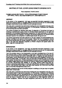
Initial calibration procedure The first ADP image (Fig. 2) was acquired on 5th May 1996 of a field of winter barley cv.

Intro (Hordeum vulgare L.). Visual interpretation identified three levels of variation: (1)

a dominating striping effect between tramlines, attributed to an uneven application of nitrogen fertilizer from a spinning-disc spreader;

(2)

a low-frequency, field-scale variation from east to west – somewhat masked by the striping; and

(3)

localised crop damage attributed to grazing rabbits, glyphosate drift and possible slug damage, all characterised by moderate to severe patches of bare soil.

Sample analyses were conducted at four sites, A, B, C and D, shown in Fig. 2, to quantify the across field variation. At each of these four sites a grid of 25 quadrats comprising a matrix five positions each with five replications which were aligned as shown in Fig. 2. These were used to assess the localised variation and the between-tramline striping effect. The shoot population was measured in each of hundred 0.25 m2 quadrats. The locations of the sample sites were fixed by ground measurement relative to the tramline system, which was clearly visible in the ADP images. Equivalent NDVI values were extracted from the images.

3.1. Results of the initial calibration. The relationship between the NDVI values derived by ADPand ground measurements of shoot population for the individual quadrat positions (four sites, each with 25 quadrats) in Fig. 4 shows a significant linear trend (probability