Building Interest Rate Curves and SABR Model Calibration by

Jeffrey Ted Johnattan Mbongo Nkounga

Thesis presented in partial fulfilment of the requirements for the degree of Master of Science in Mathematics in the Faculty of Science at Stellenbosch University

Department of Mathematical Sciences, Mathematics Division, University of Stellenbosch, Private Bag X1, Matieland 7602, South Africa.

Supervisor: Prof. Ronnie Becker

March 2015

Stellenbosch University https://scholar.sun.ac.za

Declaration By submitting this thesis electronically, I declare that the entirety of the work contained therein is my own, original work, that I am the sole author thereof (save to the extent explicitly otherwise stated), that reproduction and publication thereof by Stellenbosch University will not infringe any third party rights and that I have not previously in its entirety or in part submitted it for obtaining any qualification.

Signature: . . . . . . . . . . . . . . . . . . . . . . . . . . . J.T. J Mbongo Nkounga November 27, 2014 Date: . . . . . . . . . . . . . . . . . . . . . . . . . . . . . . .

Copyright © 2015 Stellenbosch University All rights reserved.

i

Stellenbosch University https://scholar.sun.ac.za

Abstract In this thesis, we first review the traditional pre-credit crunch approach that considers a single curve to consistently price all instruments. We review the theoretical pricing framework and introduce pricing formulas for plain vanilla interest rate derivatives. We then review the curve construction methodologies (bootstrapping and global methods) to build an interest rate curve using the instruments described previously as inputs. Second, we extend this work in the modern post-credit framework. Third, we review the calibration of the SABR model. Finally we present applications that use interest rate curves and SABR model: stripping implied volatilities, transforming the market observed smile (given quotes for standard tenors) to non-standard tenors (or inversely) and calibrating the market volatility smile coherently with the new market evidences. Keywords: credit crunch/crisis, credit risk, counterparty risk, collateral, CSA, interest rates, negative rates, Libor, Euribor, Eonia, forward curve, discount curve, single-curve, multiple-curve, interest rate derivatives, Deposit, FRA, Futures, OIS, IRS, basis swap, interpolation, global methods, bootstrapping, caps, swaptions, volatility, SABR, calibration.

ii

Stellenbosch University https://scholar.sun.ac.za

Acknowledgements First, I would like to express my sincere gratitude to my supervisor, Prof. Ronnie Becker, for his invaluable support, continuous guidance, meticulous suggestions and astute criticism and corrections, and for his inexhaustible patience throughout this thesis. Second, I would like to extend my deepest appreciation to AIMS for this tremendous opportunity and for the financial support. I would also like to extend my appreciation to ACQuFRR members for various scientific exchanges. Third, I would like to express my thanks to Marco Bianchetti and to Dr. Jöerg Kienitz for answering many of my questions and for keeping me abreast on the scientific developments around my thesis’s topic. Furthermore, I am very very thankful to Daniel J. Duffy and Andrea Germani for assisting me in C# codes, Tran, H. Nguyen and Weigardh, Anton for their assistance regarding Matlab codes, and to QuantLib (Open Source) community, especially Luigi Ballabio, for their assistance as far as C++ coding is concerned. Last but not the least, I would like to express my heartfelt thanks to my family, for their prayers, patience, love, encouragement, moral support and blessings. Your Jeffrey is progressing step by step. I would also like to extend my indebtedness to those who are no longer with us on this earth. How can we forget the Almighty God, the Father of our Lord Jesus Christ in Heaven? We put our trust in You. We praise You, we are grateful, we thank You, we love You. I will be what people think or say about me, only if I believe it.

iii

Stellenbosch University https://scholar.sun.ac.za

Dedications

To my family, relatives and friends. A big group with big hearts and strong beliefs.

iv

Stellenbosch University https://scholar.sun.ac.za

Contents Declaration

i

Abstract

ii

Acknowledgements

iii

Dedications

iv

Contents

v

List of Figures

vii

List of Tables

viii

Nomenclature

ix

1 Introduction

1

2 Single Curve 2.1 Introduction . . . . . . . . . . . . . 2.2 Definitions and notation . . . . . . 2.3 Single curve framework . . . . . . . 2.4 Curve construction mechanism . . . 2.5 Options caps, floors and swaptions 2.6 Summary and conclusion . . . . . .

. . . . . .

3 3 3 8 14 23 26

. . . . .

27 27 28 31 42 43

4 The SABR Model 4.1 Introduction . . . . . . . . . . . . . . . . . . . . . . . . . . . . 4.2 The SABR Model: description . . . . . . . . . . . . . . . . . .

44 44 47

. . . . . .

. . . . . .

. . . . . .

3 Multi-Curves 3.1 Introduction . . . . . . . . . . . . . . . . 3.2 Pricing valuation after the credit crunch 3.3 Multi curve framework . . . . . . . . . . 3.4 Options caps, floors and swaptions . . . 3.5 Summary and conclusion . . . . . . . . .

v

. . . . . .

. . . . .

. . . . . .

. . . . .

. . . . . .

. . . . .

. . . . . .

. . . . .

. . . . . .

. . . . .

. . . . . .

. . . . .

. . . . . .

. . . . .

. . . . . .

. . . . .

. . . . . .

. . . . .

. . . . . .

. . . . .

. . . . . .

. . . . .

Stellenbosch University https://scholar.sun.ac.za

vi

CONTENTS

4.3 4.4 4.5 4.6

Model dynamics . . . . . . . . . Refinement of the SABR model Calibration of the SABR model Summary and conclusion . . . .

. . . .

. . . .

. . . .

. . . .

. . . .

. . . .

. . . .

49 60 61 72

5 Interest rate curves and SABR calibration applications 5.1 Introduction . . . . . . . . . . . . . . . . . . . . . . . . . . . . 5.2 Swaption smile and SABR functional form . . . . . . . . . . . 5.3 Summary and conclusion . . . . . . . . . . . . . . . . . . . . .

73 73 74 76

6 Conclusion

77

Appendices

79

A Numéraire change

80

B Day Count Conventions

82

C Interpolation and LMA C.1 Linear interpolation . . . . . . . . . . . . . . . . . . . . . . . . C.2 Cubic splines . . . . . . . . . . . . . . . . . . . . . . . . . . . C.3 Levenberg-Marquardt algorithm . . . . . . . . . . . . . . . . .

83 83 84 86

D Data D.1 Interest rate data . . . . . . . . . . . . . . . . . . . . . . . . . D.2 Swedish market (swaption) data . . . . . . . . . . . . . . . . .

88 88 90

E Interest rate E.1 FRA . . E.2 Futures E.3 IRS . . . E.4 OIS . . . E.5 IRBS . .

. . . . .

93 93 94 95 96 98

F Analysis of the SABR Model F.1 Singular Perturbation theory . . . . . . . . . . . . . . . . . . . F.2 Scaling . . . . . . . . . . . . . . . . . . . . . . . . . . . . . . . F.3 Application of perturbation theory to SABR model . . . . . .

99 99 102 103

G Fourier transform

120

H Computer code H.1 SABR model . . . . . . . . . . . . . . . . . . . . . . . . . . . H.2 Yield curves via Quantlib . . . . . . . . . . . . . . . . . . . .

122 122 129

List of References

134

derivatives pricing formulas . . . . . . . . . . . . . . . . . . . . . . . . . . . . . . . . . . . . . . . . . . . . . . . . . . . . . . . . . . . . . . . . . . . . . . . . . . . . . . . . . . . . . . . . . . . . . . .

. . . .

. . . . .

. . . .

. . . . .

. . . .

. . . . .

. . . .

. . . . .

. . . .

. . . . .

. . . .

. . . . .

. . . .

. . . . .

. . . .

. . . . .

. . . .

. . . . .

. . . .

. . . . .

Stellenbosch University https://scholar.sun.ac.za

List of Figures 2.1 2.2 2.3 2.4 2.5 3.1 3.2 3.3 3.4 3.5

4.1 4.2 4.3 4.4 4.5 4.6 4.7 4.8 4.9 4.10 4.11 4.12 4.13 4.14 4.15 4.16

Interest Rate Swap cash flows . . . . . . . . . . . . . . . . . . . . Interest rate swap between Companies A and B . . . . . . . . . . 3M-Forward curve up to 50 years . . . . . . . . . . . . . . . . . . Top panel: 6M-Forward curve up to 60 years, bottom panel: Effect of data on the forward single curve . . . . . . . . . . . . . . . . . Effect of data on the forward single curve . . . . . . . . . . . . . .

9 10 20

3m Euribor-Eonia, Basis Swap between different tenor. . . . . . . EONIA 3M-Forward curve up to 2 years . . . . . . . . . . . . . . Top panel: EONIA 3M-Forward curve up to 30 years, bottom panel: Euribor 6M-Forward curve up to 30 years . . . . . . . . . . Top panel: Euribor Discount curve up to 30 years, bottom panel: effect of data on the forward curve using different interpolation . Top panel: effect of data on the forward curve using different interpolation, bottom panel:comparing discount curve: Euribor vs EONIA . . . . . . . . . . . . . . . . . . . . . . . . . . . . . . . .

30 38

Call’s volatility smile . . . . . . . . . . . . . . . . . . . . . . . . . Volatility smile from data in Table D.2. Red dots: market volatility. Dynamics of the parameter β . . . . . . . . . . . . . . . . . . . . Dynamics of the parameter ρ . . . . . . . . . . . . . . . . . . . . Dynamics of the parameter ν . . . . . . . . . . . . . . . . . . . . Dynamics of the parameter α . . . . . . . . . . . . . . . . . . . . Volatility smile shifting f . . . . . . . . . . . . . . . . . . . . . . Shifting f in the backbone for β = 0 . . . . . . . . . . . . . . . . Shifting f in the backbone for β = 1 . . . . . . . . . . . . . . . . 5Y12Y Calibration with different beta using Methods 1 and 2 . . 1M5Y Calibration with different beta using Method 1 and 2 . . . 5Y12Y swaption calibration using Methods 1 and 2 . . . . . . . . 1M5Y swaption calibration using Method 1 and 2 . . . . . . . . . 1M4Y swaption calibration using Method 1 for β = 0.5 and 1 . . 20Y4Y swaption calibration using Method 1 for β = 0.5 and 1 . . 1M20Y and 20Y20Y swaption calibration using Method 1 for β = 0.5.

44 45 53 54 55 56 57 58 59 63 64 66 67 69 70 71

vii

21 22

39 40

41

Stellenbosch University https://scholar.sun.ac.za

List of Tables 2.1

Data selected from Appendix D (D.1) . . . . . . . . . . . . . . . .

17

4.1 4.2 4.3 4.4 4.5 4.6 4.7

Comparison of I 0 term Hagan vs Berestycki Method 1 estimated for different beta . . . . . . Method 2 estimated for different beta . . . . . . Different methods calibrated when beta is 0 . . Different methods calibrated when beta is 0.5 . Different methods calibrated when beta is 1 . . Some swaptions calibrated with Method 1 . . .

. . . . . . .

61 61 62 65 65 65 68

D.1 EUR Deposit strip . . . . . . . . . . . . . . . . . . . . . . . . . . D.2 EUR FRA strips on Euribor 3M, Euribor 6M, and Euribor 12M. . D.3 Hull-White parameters values for Futures 3M convexity adjustment as of 11 Dec. 2012. . . . . . . . . . . . . . . . . . . . . . . . . . . D.4 EUR Futures on Euribor 3M . . . . . . . . . . . . . . . . . . . . . D.5 EUR IRS on Euribor 6M . . . . . . . . . . . . . . . . . . . . . . . D.6 EUR IRS on Euribor 3M . . . . . . . . . . . . . . . . . . . . . . . D.7 EUR IRS on Euribor 1M . . . . . . . . . . . . . . . . . . . . . . . D.8 EUR OIS . . . . . . . . . . . . . . . . . . . . . . . . . . . . . . . D.9 EUR IRBS . . . . . . . . . . . . . . . . . . . . . . . . . . . . . .

88 88

viii

. . . . . . .

. . . . . . .

. . . . . . .

. . . . . . .

. . . . . . .

. . . . . . .

. . . . . . .

. . . . . . .

. . . . . . .

89 89 89 89 90 90 90

Stellenbosch University https://scholar.sun.ac.za

Nomenclature Notation and Abreviations ω Event or outcome Ω Sample space that consists of all possible outcome F Event space P Probability measure (Ω, F, P) Probability space σ σ-algebra ∗ T Maximum fixed time horizon for all market activities {Ft }t∈[0,T ∗ ] Flow of information at time t rt Interest rate at time t Bt Bank Account at time t P (a, b) Zero Coupon Bond at time a for the maturity b L(a, b) Simply-compounded spot interest rate (Libor rate) at time a for the maturity b δ(a, b) Time interval between time a and b (according to day convention) F (t, S, T ) Simply-compounded forward interest rate K Fixed rate N Notional amount f (a, b) Instantaneous forward interest rate at time a for the maturity b QB Measure under numéraire B. T Q Measure under numéraire P (t, .) ET h Expectation under the T-forward measure i QB E . Ft Conditional expectation under the measure QB on the Ft σ-field T Fixed leg schedule S Floating leg schedule Sα,β (t) Forward Swap Rate Cs Yield curve Fs (t; Tj−1 , Tj ) s-Forward interest rate Capt Cap price at time t ix

Stellenbosch University https://scholar.sun.ac.za

NOMENCLATURE

Φ(.) Standard Normal cumulative distribution function Floort Floor price at time t S(t, k, n) ATM strike σi Volatility of the Caplet/Flooret between time interval [Ti−1 , Ti ] 

a−b

+

max(a − b, 0)

CyP (t0 ) Discount yield Curve CyF (t0 ) y-Forward yield Curve ry y-Interest rate By (t) Bank Account under y-Interest rate dcz Corresponding day count convention for the zero coupon rate Ty y Fixed leg schedule Ly,j Spot Libor rate fixed on the market at time Tj−1 FRAStd Standard Forward Rate Agreement Depo(Tj ; Tj ) Payoff of the lender in an interest rate Deposit RyDepo (T0F ; Tj ) y-Simply-compounded Deposit interest rate FRAMkt Market Forward Rate Agreement RyF ut (t; T) y-Simply-compounded Future interest rate CyF ut (t; Tj−1 ) Convexity adjustment Futures(t; T) Futures payoff at payment IRSletfloat Float coupon payoff Interest Rate Swap IRSletfix Fixed coupon payoff Interest Rate Swap Ac (t; S) Annuity Swap discounted with Pc (t, .) OIS Ron Equilibrium OIS rate Cc (T0 ) OIS Yield Curve at time T0 SABR Stochastic Alpha Beta Rho CMS Constant Maturity Swap sse Sum Squared Error β Exponent for the forward rate α Initial variance ν Volatility of variance ρ Correlation between the two Wiener processes K Strike price F Forward rate of a log-normal underlying with constant r Risk-free interest rate σB Black-Scholes constant volatility tex Time to maturity mkt σj Market volatilities

x

Stellenbosch University https://scholar.sun.ac.za

Chapter 1 Introduction Before the 2007-2008 credit crunch, the single curve approach was predominantly in use for consistently pricing financial instruments. This approach has received less interest in the current literature, perhaps this is because the framework has become obsolete nowadays. Nevertheless, we can refer to Duffy and Germani (2013, Chapter 15). A more detailed literature review can be found in Chapter 2. In contrast, the multi-curve approach has received a lot of interest in the recent literature. In particular, we can find more information in Duffy and Germani (2013, Chapter 16), Ametrano and Bianchetti (2009), Ametrano and Bianchetti (2013) and others (we refer to Chapter 3 for a more detailed literature review). The Black-Scholes model is based on the assumption of constant volatility cannot incorporate the volatility smiles usually observed in the markets. Therefore, we must consider alternative stochastic volatility models such as the SABR model. The SABR model was first introduced by Hagan et al. (2002). This model has received a lot of attention in the recent literature. Different authors have contributed to its extension and to its improvement. We can cite the works of Oblój (2008) and others (we refer to Chapter 4 for a more detailed literature review).

Problem statement and limitations Using the SABR model, Mercurio and Pallavicini (2006) proposed a very simple procedure for stripping consistently implied volatilities and CMS adjustments from the market quotes of swaption smiles and CMS swap spreads. Their approach was done in the single-curve framework. We aim to propose an extension of their approach in the multi-curve framework, but we only deal with a method for stripping consistently implied volatilities from the market quotes of swaption smiles. This work is inspired mainly by Bianchetti and Carlicchi (2011) and Kienitz (2013). 1

Stellenbosch University https://scholar.sun.ac.za

CHAPTER 1. INTRODUCTION

2

To achieve this, we start by reviewing the traditional pre-credit crunch approach that considers a single curve to consistently price all instruments. We then review the curve construction methodologies (bootstrapping and global methods) to build an interest rate curve. Then, we extend this work in the modern post-credit framework. Furthermore, we review the calibration of the SABR model and we highlight the procedure of the calibration after the crisis.

Thesis outline The thesis is organized as follows. Chapter 2 presents the methodologies (Bootstrapping and Best Fit) for constructing interest rate curves (discounting and forward yield curves), accompanied by their implementation. It reviews the fundamental pricing formulas for plain vanilla interest rate derivatives in the classical framework with no collateral. Chapter 3 gives an overview of a number of changes that have taken place in the financial markets since the credit crunch of 2007. It introduces the use of multiple distinct curves to ensure market coherent estimation of discount factors and of forward rates with different underlying rate tenors. Chapter 4 reviews the calibration of the SABR model for different swaptions. It presents two different methods (with and without refinement), and shows that the SABR model accurately captures the volatility smiles in the markets. Moreover, this chapter reveals the complexity of the market after the credit crunch. Chapter 5 presents applications that use interest rate curves and SABR model such as: stripping implied volatilities, transforming the market observed smile (given quotes for standard tenors) to non-standard tenors (or inversely) and calibrating the market volatility smile coherently with the new market evidences. Finally, the summary and conclusion of the thesis is presented in Chapter 6. The data used in this thesis can be found in Appendix D, also a summary code and more details and proofs of some formulae presented can be found in Appendices A, B, C, E, F, G and H.

Stellenbosch University https://scholar.sun.ac.za

Chapter 2 Single Curve 2.1

Introduction

Generally, to trade financial instruments, we need to discount a set of cash flows occurring in the future or to estimate spot rates, forward rates for financial transactions taking place in the future. The best way to achieve all these is to construct an interest rate curve. In the finance market, there are two frameworks for interest rate curve, mainly: Single Curve and Multi or Multiple Curves. The Single Curve represents the traditional or pre-credit crunch approach, which considers a unique curve for both forwarding and discounting. However, after the 2007-2008 credit crunch, a unique curve for both forwarding and discounting is no longer consistent (we will discuss this in Chapter 3). Consequently, new approaches have begun to rise and to be used and the Single Curve framework was superseded by the Multi-Curve framework. In this chapter, we will provide some basics definitions and necessary concepts that we need later to explain the mechanism of the construction of curves. We assume that there is no default risk in the interbank (default risk and inconsistency between different instruments are ignored in this chapter).

2.2

Definitions and notation

Let (Ω, F, P, Ft ) be a filtered probability space describing the market, where: • Ω is the sample space that consists of all possible outcome ω ∈ Ω. • F is the event space. It is a σ-algebra consisting of subsets (events) of the sample space X ⊆ Ω. • P is the probability measure on the sample Ω. For any event X ⊆ Ω, P(X) is the probability of X occurring.

3

Stellenbosch University https://scholar.sun.ac.za

4

CHAPTER 2. SINGLE CURVE

Let T ∗ be the maximum fixed time horizon for all market activities. The filtration {Ft }t∈[0,T ∗ ] (that consists of a family of increasing σ-algebras) represents a flow of information at time t. We have: • For any a < b < T ∗ we have Fa ⊆ Fb ⊆ FT ∗ ≡ F. • F0 = {∅, Ω}. Definition 2.1. A term structure of interest rates is a set of interest rates sorted by time to maturity. The curve shows the relation between the (level of) interest rate (or cost of borrowing) and the time to maturity. We can build several types of curves using rates of a different nature, for example zero coupon yield curve, forward rates curve, instantaneous forward curve. Below we provide basic mathematics formulae to deal with these term structures of interest rates. Definition 2.2 (Bank Account). Let rt be a positive stochastic function of time and which models the short term interest rate. At time t > 0, the value of a bank account is defined by Bt . We assume that the evolution of the bank account satisfies the following differential and initial condition: dBt = rt Bt dt,

B0 = 1.

(2.2.1)

By simple integration, equation (2.2.1) gives Bt = exp

!

t

Z 0

∀ t ∈ [0, T ∗ ].

rs ds

(2.2.2)

Definition 2.3 (Zero-Coupon Bonds). A T-maturity zero-coupon bond also called a pure discount bond or a T-bond, is a contract that guarantees its holder the payment of one unit of currency at time T , with no intermediate payments. At time t 6 T , the contract value is P (t, T ). It follows that P (T, T ) = 1 for all T 6 T ∗ . Using formula (A.0.1), when the bank account Bt is taken as the numéraire (i.e. Nt = Bt ), then QN = QB and S(t) = P (t, T ). It follows that "



#

1 P (t, T ) B = EQ Ft . Bt BT

(2.2.3)

From equation (2.2.3), we have P (t, T ) = E

QB

"

exp −

Z t

T

! # ru du Ft

∀ t ∈ [0, T ].

(2.2.4)

Stellenbosch University https://scholar.sun.ac.za

5

CHAPTER 2. SINGLE CURVE

Definition 2.4 (Simply-compounded spot interest rate). The simply-compound spot interest rate L(t, T ) is the constant rate defined by L(t, T ) =

1 − P (t, T ) δ(t, T )P (t, T )

(2.2.5)

where δ(t, T ) is the time interval between time t and T (accrual factor according to the day convention chosen1 ). The notation L is motivated by the fact that the market Libor2 rates are simply-compounded rates. Justification Equation (2.2.5) can be explained as follows: we note L(t, τ ) the Libor rate at time t, of tenor τ 3 . At time t, if one lends 1 at Libor, then at time t + τ , one receives back 1 + δL (t, t + τ )L(t, τ ), where δL (t, t + τ ) is the actual time (day count convention) between times t and t + τ . To avoid arbitrage (ignoring credit issues), we must have h

i

1 + δL (t, t + τ )L(t, τ ) P (t, t + τ ) = 1.

(2.2.6)

Equation (2.2.5) follows from this last expression. Definition 2.5 (The T-Forward measure). The forward martingale measure (or briefly, the T-Forward measure) QT , corresponding to the zero coupon bond P (t, T ) maturing at time T is an equivalent probability measure to QB on (Ω, FT ), and is defined via the Radon-Nikodým derivative given by ηT =

BT−1 1 B0 P (T, T ) dQT = = = , B −1 dQB P (0, T )BT P (0, T )BT EQ [BT ]

QB -a.s..

(2.2.7)

Proposition 2.6. The relative prices, for t 6 U < T , P (t, U )/P (t, T ) are martingales under QT .

Forward Rates Forward rates are characterized by three time instants: the current time t at which the rate is considered, the settlement date S and its maturity T with t < S 6 T . Forward rates are interest rates applicable to a financial transaction that will take place in the future. We can define a forward rate through a (prototypical) forward-rate agreement (FRA). 1

we refer to Appendix B for more details Libor is the abbreviation of London Interbank Offered Rate, it is the average interest rate at which a group of bank in the London market lend money to one another and it is offered in ten major currencies . 3 The tenor of interest rate is its maturity period, the period from the point of investment to the time that interest is paid. 2

Stellenbosch University https://scholar.sun.ac.za

6

CHAPTER 2. SINGLE CURVE

Definition 2.7 (FRA). A FRA is contract in which two counterparties agree to exchange two streams of cash flows in the same currency and in which the notional principal N remains constant over the life of the contract. In the contract, one party pays an interest rate based on the spot rate L(S, T ) and receives a fixed rate K. Formally, at time T one receives N δ(S, T )K units of currency and pays the amount N δ(S, T )L(S, T ) (assuming the same day-count conventions for both parties). The value of the contract at time T is therefore: h

i

N δ(S, T ) K − L(S, T ) . Using equation (2.2.5), the value of the contract at time T can be written as

"

#

1 N δ(S, T )K − +1 . P (S, T ) The value of the contract at time t, using equation (A.0.2), is QT

P (t, T )E

"

1 +1 N δ(S, T )K − P (S, T ) 

 # Ft .

This leads to h

i

QT



#



#

"

1 F t . P (S, T )

"

P (S, S) F t . P (S, T )

P (t, T )N δ(S, T )K + 1 − P (t, T )N E Using the fact that 1 = P (S, S), we have h

i

QT

P (t, T )N δ(S, T )K + 1 − P (t, T )N E

Using Proposition 2.6, P (S, S)/P (S, T ) are martingales under QT , therefore the total value of the contract at time t is h

i

FRA(t, S, T, δ(S, T ), N, K) = N P (t, T )δ(S, T )K − P (t, S) + P (t, T ) . (2.2.8)

There is one value of K that ensures that the value of the contract at time t is 0. The resulting rate is called the simply-compounded forward rate and which we define below. Definition 2.8 (Simply-compounded forward interest rate). At time t, the current time or the date today, we fix two future points S and T such that t < S 6 T , where S is called settlement date and T is called time to maturity, the simply-compounded forward interest rate F (t; T, S) for [S, T ] contracted at time t, is defined by: !

P (t, S) 1 F (t; S, T ) = −1 . δ(S, T ) P (t, T )

(2.2.9)

Stellenbosch University https://scholar.sun.ac.za

7

CHAPTER 2. SINGLE CURVE

Hence, using equation (2.2.8), the value of the FRA can be written as h

i

FRA(t, S, T, δ(S, T ), N, K) = N P (t, T )δ(S, T ) K − F (t; S, T ) .

(2.2.10)

Definition 2.9 (Instantaneous forward interest rate). The instantaneous forward interest rate, f (t, T ), contracted at time t for the maturity T > t is defined by ∂ ln P (t, T ) f (t, T ) = lim+ F (t; T, S) = − . (2.2.11) S→T ∂T The last equality follows from assuming that δ(S, T ) = T − S, for small T −S 1 P (t, T ) − P (t, S) S→T P (t, S) S−T 1 ∂P (t, T ) =− P (t, T ) ∂T ∂ ln P (t, T ) . =− ∂T

lim+ F (t; T, S) = − lim+

S→T

We consider also the following proposition. Proposition 2.10. A simply-compounded forward rate spanning a time interval ending in T is a martingale under the T -forward measure, i.e. E

QT

# F (v; S, T ) Ft = F (t; S, T ),

"

0 6 t 6 v 6 S < T.

(2.2.12)

In particular, the forward rate spanning the interval [S, T ] is the QT -expectation of the future simply-compounded spot rate at time S for the maturity T, i.e. E

QT

# L(S, T ) Ft = F (t; S, T ),

"

0 6 t 6 S < T.

(2.2.13)

Definition 2.11 (Swap). A swap contract is the exchange between two counterparties, with no notional amount exchanged, of cash-flows (interest rates, or currencies). The agreement defines the dates when the cash flows are to be paid and the way in which they are to be calculated. There are many types of swaps. Among them we can cite: Interest Rate Swaps, Currency Swaps, Credit Swaps, Commodity Swaps. Later on, we will discuss some of them, such as: Interest Rate Swap (IRS), Overnight Indexed Swap (OIS), Interest Rate Basis Swap (IRBS). In a swap, the individual future cash flows that are swapped are called legs (there are: fixed legs and floating legs) which are calculated over a notional principal amount. In an interest rate swap for instance, usually there is one counterparty which agrees to pay the fixed rate and the other one which agrees

Stellenbosch University https://scholar.sun.ac.za

CHAPTER 2. SINGLE CURVE

8

to pay the floating rate (Libor rate for example) over the period, or an adjusted Libor rate (we will assume this in what follows). The fixed or floating rate is multiplied by a notional principal amount and an accrual factor given by the appropriate day count convention. Definition 2.12 (Over-the-counter market). Over-the-counter (OTC) market is a decentralized market, without a central physical location, where market participants trade with one another through various communication modes such as the telephone, email and proprietary electronic trading systems. Definition 2.13 (Collateral). Collateral consists of providing an item as a security against the possibility of payment default by the counterparty in a contract.

Yield curves notation We denote by Cy the yield curve defined in a form of continuous term structure or discount factors (or zero coupon bonds) CyP (t0 ) = {T −→ Py (t0 , T ), T > t0 }, or forward rates CyF (t0 ) = {T −→ Fy (t0 ; T, T + y), T > t0 } with t0 being a reference date of the curves (e.g. settlement date, sport date, or today). The subscript or index y corresponds to tenor, i.e. y ∈ {OIS, 1M, 2M, 3M, 6M, 12M }.

2.3

Single curve framework

In this section we introduce the curve construction mechanism to build an interest rate curve. After having introduced the idea of the interest rate curve, we give a basic overview of the instruments used as inputs as well as the main methods used in curve building such as bootstrapping and global methods.

2.3.1

Market instruments selection

There are different types of instruments that can be selected for constructing an interest yield curve, and it is impossible to include all available instruments in the market. Therefore it is important to make a very careful selection of these elements and to minimize the mispricing level of the excluded instruments. In the selection, the priority is given to more liquid4 instruments such as: 4

The features of the liquid asset are: rapidity to be sold, minimal loss of value, any time within the market hours.

Stellenbosch University https://scholar.sun.ac.za

9

CHAPTER 2. SINGLE CURVE

Deposits, Forward rate agreements, futures, swaps, etc. We describe these market instruments in detail below. 2.3.1.1

Interest Rate Swaps (IRS)

Interest Rate Swaps are OTC contracts in which two counterparties agree to exchange interest rate cash flows, based on a specified notional amount from a fixed rate to a floating rate (or vice versa) or from one floating rate to another. They are generally used to manage exposure to fluctuations in interest rates. The illustration is given bellow on Figure 2.1, where the upward pointing arrows are positive cash flows (fixed rate) and the downward pointing arrows are negative cash flows (floating rate). The gray arrows represent the exchanged amount for each period.

Figure 2.1: Interest Rate Swap cash flows. Blue arrows are cash flows (fixed rate) and red arrows are cash flows (floating rate), the gray arrows are the exchanged amount.

Tables D.5, D.6, D.7, in this order, report the quoted swaps 1M, 3M, 6M Euribor rates. These cash flows are typically tied to a floating Libor rate L(Tj−1 , Tj ) versus a fixed rate K, therefore the IRS is characterised by the following schedule T = {T0 , T1 , . . . , Tn }, S = {S0 , S1 , . . . , Sm }, S0 = T0 , Sn = Tm .

floating leg schedule, fixed leg schedule,

Stellenbosch University https://scholar.sun.ac.za

10

CHAPTER 2. SINGLE CURVE

and coupon payoffs are IRSletfloat (Tj ; Tj−1 , Tj , L) = N L(Tj−1 , Tj )δL (Tj−1 , Tj ), j = 1, . . . , n (2.3.1) IRSletfix (Si ; Si−1 , Si , K) = N KδK (Si−1 , Si ), i = 1 . . . , m where δK (Si−1 , Si ) is the fix leg time interval between Si−1 and Si and δL (Tj−1 , Tj ) is the floating leg time interval between Tj−1 and Tj . The coupon payoffs at time t, using equations (A.0.2) and (2.2.13), are given by IRSletfloat (t, Tj ; Tj−1 , Tj , L) = N P (t; Tj )F (t; Tj−1 , Tj )δL (Tj−1 , Tj ), IRSletfix (t, Si ; Si−1 , Si , K) = N KP (t; Si )δK (Si−1 , Si ). The present value of the fixed leg, at time t, therefore is given by P Vfixed (t) = K × N ×

m X

P (t; Si )δK (Si−1 , Si )

(2.3.2)

i=1

and the present value of the floating leg, at time t, is given by P Vfloat (t) = N ×

n X

P (t; Tj )F (t; Tj−1 , Tj )δL (Tj−1 , Tj ).

(2.3.3)

j=1

Using equation (2.2.9), the sum in equation (2.3.3) can then be simplified as follows n X

P (t; Tj )F (t; Tj−1 , Tj )δL (Tj−1 , Tj ) = P (t; T0 ) − P (t; Tn ).

(2.3.4)

j=1

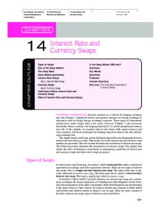
However, we will see in the next chapter, this will not be possible in the modern multiple-curve framework. Furthermore, because IRS are traded OTC contracts; formula (A.0.3) will be used instead of formula (A.0.2). Example 2.14. Company A and Company B want to borrow a certain amount of money each at the lowest possible cost for a certain period with annual compounding. Company A expects interest rates to decline and wants floating rate borrowing, while Company B expects interest rates to rise and wants to lock-in the fixed rate available to it. Floating Rate: LIBOR + 1% Company A

Company B Fixed Rate: 6%

Figure 2.2: Interest rate swap between Companies A and B

Stellenbosch University https://scholar.sun.ac.za

11

CHAPTER 2. SINGLE CURVE

Forward Swap Rate The forward swap rate Sα,β (t) at time t is the value of K that causes the contract to have zero value at time t, i.e. such that P Vfloat (t) = P Vfixed (t), we have: P (t, Sα ) − P (t, Sβ ) Sα,β (t) = Pβ . (2.3.5) j=α+1 δj,j−1 P (t, Tj ) 2.3.1.2

Overnight Indexed Swap (OIS)

An Overnight Indexed swap (OIS) is an agreement between two counterparties to exchange at each payment date or at maturity the difference between fixed rate and floating rate on the nominal amount. The periodic floating rate is equal to the geometric average of an overnight rate over every day of the payment period. For the EUR market the fixing is named EONIA (EUR Overnight Index Average). The principal is not exchanged between counterparties at the end of the trade. The OIS coupon payoffs are given by OISletfloat (Tj ; Tj , Ron ) = N Ron (Tj ; Tj )δon (Tj−1 , Tj ) j = 1, . . . m, OISletfix (Si ; Si−1 , Si , K) = IRSletfix (Si ; Si−1 , Si , K) i = 1, . . . n,

(2.3.6)

where Ron (Tj ; Tj ) is the coupon rate compounded from over night rates over the j−th coupon period (Tj−1 , Tj ) and it is given by Ron (Tj ; Tj ) :=

"

1 δ(Tj−1 , Tj )

nj Y

#

[1 + R(Tj,k−1 , Tj,k )δ(Tj,k−1 , Tj,k )] − 1

k=1

where Tj = {Tj,0 , . . . , Tj,nj }, is the sub-schedule for the coupon rate R(Tj , Tj ), and R(Tj,k−1 , Tj,k ) are the single over night rate spanning the over night time Snj (Tj,k−1 , Tj,k ) intervals (Tj,k−1 , Tj,k ). We have also Tj,0 = Tj−1 , (Tj−1 , Tj ) = k=1 and Tj,nj = Tj , for j = 1, . . . , n. The price and equilibrium rate of the OIS is given, in Appendix E (equations (E.4.9) and (E.4.10)), by h

i

c OIS OIS(t; T, S, Ron , K, ω) = N ω Ron (t; T, S) − K Ac (t; S)

and Pm

RxOIS (t; T, S)

Pc (t; Tj )Ron (t; Tj )δon (Tj−1 , Tj ) Ac (t; S) Pc (t; T0 ) − Pc (t; Tm ) = Ac (t; S) =

j=1

(2.3.7)

where Ac (t; S) =

n X i=1

Pc (t; Si )δK (Si−1 ; Si ).

(2.3.8)

Stellenbosch University https://scholar.sun.ac.za

12

CHAPTER 2. SINGLE CURVE

In Table D.8, we have a report of the OIS on Eonia from 1W to 60Y which starts at T0 = today + 2 business and we notice very low and negative quotations for short term OIS. Considering the OIS schedule Tj = {T0 , . . . , Tj } = Sj , equation (2.3.7) gives Pc (t; T0 ) − Pc (t; Ti−1 ) OIS . Ron (T0 ; Ti−1 ) = Ac (T0 ; Ti−1 ) From equation (2.3.8), we have Ac (T0 ; Ti ) = Ac (T0 ; Ti−1 ) + Pc (T0 ; Ti )δK (Ti−1 ; Ti ). OIS OIS Using the expression of Ron (T0 ; Ti ), Ron (T0 ; Ti−1 ) and Ac (T0 ; Ti−1 ) above, P the discount curve Cc (T0 ) at time Ti is given by

h

Pc (T0 ; Ti ) =

i

OIS (T ;T OIS Ron 0 i−1 )−Ron (T0 ;Ti )

Ac (T0 ;Ti )+Pc (T0 ;Ti−1 )

. (2.3.9)

OIS (T ;T )δ (T 1+Ron 0 i K i−1 ;Ti )

Using equations (2.2.9) and (2.3.9), the forward curve CcF (T0 ) at time Ti is given by

Fc (T0 ; Ti−1 , Ti ) = 2.3.1.3

h

 

1 h δon (Ti−1 ;Ti ) 

i

 

OIS (T ;T )δ (T Pc (T0 ;Ti ) 1+Ron 0 i K i−1 ;Ti )

i

OIS (T ;T OIS Ron 0 i−1 )−Ron (T0 ;Ti ) Ac (T0 ;Ti−1 )+Pc (T0 ;Ti−1 )

− 1.

Deposits

Interest rate deposits (Depos) are standard money market zero coupon contracts. The lender pays the amount N to the borrower at time T0 and at maturity Tj the borrower pays back to the lender the amount N plus the interest accrued over the period [T0 , Tj ] at the simply compounded Deposit rate RyDepo (T0F ; Tj ), fixed at time T0F ≤ T0 . We have the contract schedule {T0F , T0 , Tj }. For the lender, the payoff at maturity Tj is given by 



Depo(Tj ; Tj ) = N 1 + RyDepo (T0F ; Tj )δL (T0 ; Tj ) .

(2.3.10)

Since Deposits are not traded on OTC, using equation (A.0.2), the price of the payoff at time t, satisfying T0F ≤ t ≤ Tj , is given by Depo(t; Ti ) =

Tj P (t; Tj )EQ t

"

#

Depo(Tj ; Tj )





= N P (t; Tj ) 1 +

RyDepo (T0F ; Tj )δL (T0 ; Tj )

.

(2.3.11)

Deposits rates are treated as Libor rates, so we have RyDepo (T0F ; Tj ) = L(T0 , Tj ). Table D.1 shows data on Euro Deposit from 1 day up to 1 year. The discount curve CyP (T0 ) at time Tj is obtained using the following relation Py (T0 , Tj ) =

1

1+

, RyDepo (t0 ; Tj )δL (T0 , Tj )

T0 < Tj .

(2.3.12)

Stellenbosch University https://scholar.sun.ac.za

CHAPTER 2. SINGLE CURVE

2.3.1.4

13

Futures

Futures contracts are agreements to buy or sell a stated amount of a security, currency, commodity, or a financial instrument, at a predetermined future date and price. While an option gives the holder the right to buy or sell the underlying asset at expiration, the holder of the Futures contract is obligated to fulfil the terms of his or her contract. Before the crisis, Futures were treated as FRA (Definition 2.7). We will see the change in evaluating Futures in Section 3.3.2.3. 2.3.1.5

Basis Swaps (IRBS)

Interest Rate Basis Swaps are OTC contacts in which two parties exchange two floating rate (with different tenor x and y) payments in the same or different currencies. This is usually done to limit interest-rate risk that a company faces as a result of having differing lending and borrowing rates. There are two ways of building IRBS instruments: two fixed vs floating IRS, and single IRS floating vs floating plus spread. We only treat the latter way (floating vs floating plus spread), because it is most used. IRBS as single IRS Here, the IRBS is a portfolio of a floating vs floating IRS with legs indexed to two different Libors. Tx = {Tx,0 , . . . , Tx,nx }, x leg schedule, Ty = {Ty,0 , . . . , Ty,ny }, y leg schedule, with Tx,0 = Ty,0 , Tx,nx = Ty,ny and coupon payoffs are IRBSletx = N Lx (Tx,i−1 , Tx,i )δL (Tx,i−1 , Tx,i ) 

IRBSlety = N Ly (Ty,j−1 , Ty,j ) + 4(t; Tx , Ty )]δL (Ty,j−1 , Ty,j )

(2.3.13)

with i = 1, . . . , nx ; j = 1, . . . , ny ; k = 1, . . . m and where 4(t; Tx , Ty ) in the second leg is a constant basis spread on Ly (Ty,j−1 , Ty,j ) for maturity Tx,nx = Tx,ny . The EUR market quotes standard plain vanilla Basis swap under the form aM vs bM , it is a kind of swap where we have the same fixed legs and floating legs paying Euribor aM and bM . Before the crisis, the basis spread 4(t; Tx , Ty ) was negligible. Hence IRBSletx ' IRBSlety . Therefore, for instance, for a IRBS receiving Euribor yM and paying Euribor 3M for maturity Tj , we have IRS (t, T, S). RxIRS (t, T, S) ' R3M

(2.3.14)

Stellenbosch University https://scholar.sun.ac.za

CHAPTER 2. SINGLE CURVE

14

Interpolation Interpolation is a method of constructing new data points within the range of a discrete set of known data points. In other words, it is a process of approximating the value of a function y(t) (satisfying y(τj ) = yj ) between two points at which it has prescribed values. Interpolation is very important in yield curve construction and determines some characteristics of the curve. A lot of risk and money can be hidden behind the interpolation method. There are many choices of interpolation function, however we are interested in interpolations that preserve arbitrage-free conditions, localness (a change in an input, affects the shape of the curve only locally), smoothness, positivity and stability (a change in an input, does not affect the entire shape of the curve) of forward rates. A typical headache for an interest rate trader is to choose between forward curve smoothness and bump hedge localness. Also we cannot use more than one method simultaneously (because each method satisfies specific requirement). Interpolation, as we will see in Example 2.4.5, can be used in two phases. First, directly on market quotes to complete missing information. Second, internally to return discount factors for time intervals not directly covered by information of interest rates (the interaction between these two phases is crucial). In Appendix C, we present the interpolation methods that are used in this work. More details about interpolation can be found in Hagan and West (2008) or Duffy and Germani (2013).

2.4

Curve construction mechanism

There are two main methods for curve construction starting from market data: traditional bootstrapping method and the global method. In both cases the curve building process should be calibrated to a set of quotes by solving the equations that set the theoretical values equal to the market values. Also, in both cases, we underline that interpolation is needed to complete missing data through the process of calibration.

2.4.1

Bootstrapping method

The traditional bootstrapping method consists in solving the equations that set the theoretical values equal to market values sequentially (Example 2.4.5). We assume that different instruments are associated with different dates, so that, for instance, we cannot calibrate both on a 6m deposit and a 6m swap since they would be associated with the same calibration date. Starting from shorter maturities we progress sequentially to longer maturities. In the process missing information can be retrieved using interpolation. Because the process is done

Stellenbosch University https://scholar.sun.ac.za

CHAPTER 2. SINGLE CURVE

15

sequentially, for this reason only interpolation that preserves the localness should be used (for example, the linear on the logarithm of discount factor interpolation method).

2.4.2

Best Fit method

Curve fitting is the process of constructing a curve that has the best fit to a series of data points, possibly subject to constraints. Curve fitting can involve either interpolation, where an exact fit to the data is required, or smoothing, in which a “smooth” function is constructed that approximately fits the data (for this end we may use Levenberg-Marquardt nonlinear least squares solver algorithm).

2.4.3

Single curve market instruments selection

The single curve was usually constructed based on the selection of the following market instruments5 (more information can be found in common textbooks such as: Hull (2009), Rebonato and Rebonato (1998), Chibane et al. (2009)). 1. Deposit contracts, covering the window from today up to 1Y. 2. FRA contracts, covering the window from 1M up to 2Y. 3. Futures contracts, covering the window from 3M up to 2Y and more. 4. IRS contracts, covering the window from 2Y-3Y up to 30Y. The instruments cited above are not homogeneous in the underlying rate (they admit underlying interest rates with mixed tenors).

2.4.4

Single curve bootstrapping approach

The pre-crisis standard market practice, which was based on the single-curve approach (and that can be found for instance in: Ron (2000), Ametrano and Bianchetti (2009), Bianchetti (2008), Hagan and West (2006), Ametrano (2011), Hagan and West (2008) and Andersen (2007)), can be summarised in the following steps: 1. Interbank credit/liquidity issues do not matter for pricing, Libors are good proxy for risk free rates, Basis Swap spreads are negligible (and not taken into consideration). 2. The collateral does not matter for pricing, Libor discounting is adopted. 5

also called blocks

Stellenbosch University https://scholar.sun.ac.za

CHAPTER 2. SINGLE CURVE

16

3. Select one finite set of the most convenient vanilla instrument traded on the market with increasing maturities. 4. Construct one yield curve by using the selected instruments (as in Section 2.4.3). 5. Compute on the same curve FRA rates, discounts factors by using formulae presented in Section 2.3.1 above. 6. If necessary, compute the delta sensitivity and hedge the resulting delta risk using the suggested amounts (hedge ratios) of the same set of vanillas. We emphasis that, in this framework, on a given currency, a unique yield curve is built and used to price any interest rate derivative. It goes the same way to suppose that there exists a unique underlying short rate process that is able to model and explain the whole term structure of interest rates for all tenors. In addition, the prices of a derivative are calculated relatively to a set of plain vanillas quoted on the market. Finally given the fact that discount factors and forward rates are obtained by interpolation, it follows in general that, there may exist arbitrage possibilities. General settings The reference date for the yield curve can be: today, spot date6 or in principal any business day after today. The reference date of the EUR market, except ON (OverNight i.e. between today and tomorrow) and TN (Tomorrow Next i.e. between Tomorrow and Next day) Deposit contracts, is t0 = spot date. The vector of all the dates of the curve from the reference date up to any maturity is called the Time grid or pillars or also knots. The parameter which defines the reference currency of the yield curve corresponding to the currency of the instruments is called Calendar. TARGET Business Day refers to a day on which the Trans-European Automated Real-time Gross Settlement Express Transfer (TARGET) System, or any successor thereto, is operating credit or transfer instructions with respect of payments in Euro. Business Day Convention is a procedure used for adjusting payment dates in response to days that are not TARGET Business Days. Following Business Day Convention is a procedure in which payment days that fall on a Holiday or Saturday or a Sunday roll forward to the next TARGET Business Day. On the other hand Modified Following Business Day Convention is a procedure in which payment days that fall on a Holiday or Saturday or a Sunday roll forward to the next TARGET Business Day, unless that day falls in the next calendar month, in which case the payment day rolls backward to the immediately preceding TARGET Business Day. 6

spot date of a transaction is the normal settlement day when the transaction is done today.

Stellenbosch University https://scholar.sun.ac.za

17

CHAPTER 2. SINGLE CURVE

2.4.5

Yield curve bootstrapping example

We present here an example of bootstrapping a yield curve from data market. We use the theory presented above in a more pragmatic manner. In Section 2.4.3, we have seen how to select markets instruments. Using data in Tables D.1, D.2, D.4 and D.5, we select markets instruments that we report in Table 2.1 below. In Section 2.4.4, we have presented the steps used in the bootstrapping method. The idea is to build up sequentially the yield curve from shorter maturities to longer maturities (15y in this example). The spot date t0 is 13 December, 2012 (13/12/12). The chosen day-count convention is the Actual/360, hence δ(T, S) =

Deposit (%) SN 0.040 1w 0.070 1m 0.110 2m 0.140 3m 0.180 6m 0.320

actual number of days between T and S . 360

FRA (%) FRA 2 × 5 0.141 FRA 4 × 10 0.256

18 18 19 18

Futures Sep 13 99.8725 Dec 13 99.8425 Mar 14 99.8025 Jun 14 99.7425

Swaps (%) 2y 0.324 3y 0.424 4y 0.576 5y 0.762 7y 1.135 10y 1.584 15y 2.037

Table 2.1: Data selected from Appendix D (D.1)

• The first column in Table 2.1 contains the Deposit rates for maturities {T1 , . . . , T6 } = {14/12/12, 20/12/12, 14/01/13, 13/02/13, 13/03/13, 13/06/13}.

Therefore, we have 1, 7, 32, 62, 90 and 182 days to maturity, respectively. The discount factor, using equation (2.3.12), is P (t0 , Ti ) =

1 . 1 + L(t0 , Ti )δ(t0 , Ti )

for i = 1, . . . , 6. • The second column in Table 2.1 contains the FRA rates for maturities {V1 , V2 } = {13/05/13, 15/10/13}. Note that the FRA 2 × 5 starts the 13/02/13 and matures the 13/05/13 and the FRA 4 × 10 starts the 15/04/13 and matures the 15/10/13.

Stellenbosch University https://scholar.sun.ac.za

18

CHAPTER 2. SINGLE CURVE

Therefore, we have 89 and 184 days to maturity, respectively. Then using equation (2.2.9), we have P (t0 , 13/05/13) =

P (t0 , 13/02/13) . 1 + δ(13/02/13, 13/05/13)F (t0 , 13/02/13, 13/05/13)

P (t0 , 13/02/13) = P (t0 , T4 ) is known from the previous block. Similarly, we have P (t0 , 15/10/13) =

P (t0 , 15/04/13) . 1 + δ(15/04/13, 15/10/13)F (t0 , 15/04/13, 15/10/13)

Here, however, P (t0 , 15/04/13) is unknown. This is where interpolation comes in. We can interpolate P (t0 , 15/04/13) between P (t0 , T5 ) and P (t0 , T6 ) from the previous block. • The futures are quoted as futures price (third column in Table 2.1). For settlement day Ui , we can find futures rate by using the relation 100(1 − FF (t0 ; Ui , Ui+1 )) where FF (t0 ; Ui , Ui+1 ) is the futures rate for period [Ui , Ui+1 ] prevailing at t0 , and {U1 , . . . , U5 } = {18/09/13, 18/12/13, 19/03/14, 18/06/14, 17/09/14} hence δ(Ui , Ui+1 ) = 91/360. We treat futures rates as if they were simple FRA rates (previous block), that is, we set F (t0 ; Ui , Ui+1 ) = FF (t0 ; Ui , Ui+1 ). Then using equation (2.2.9), we have P (t0 , Ui+1 ) =

P (t0 , Ui ) . 1 + δ(Ui , Ui+1 )F (t0 , Ui , Ui+1 )

By this formula, we are able to calculate the discount factor P (t0 , Ui ) for i = 2, 3, 4, 5. However, we need to calculate P (t0 , U1 ) first. Once again, interpolation is needed. We can interpolate P (t0 , U1 ) between P (t0 , V1 ) and P (t0 , V2 ) from the previous block. The linear interpolation of the discount factors is given by: P (0, T ) =

T − Tk−1 Tk − T P (0, Tk−1 ) + P (0, Tk ), Tk − Tk−1 Tk − Tk−1

for Tk−1 6 T 6 Tk . While the linear interpolation of the log discount factors is: Tk − T T − Tk−1 log P (0, T ) = log P (0, Tk−1 ) + log P (0, Tk ), Tk − Tk−1 Tk − Tk−1 for Tk−1 6 T 6 Tk .

Stellenbosch University https://scholar.sun.ac.za

19

CHAPTER 2. SINGLE CURVE

• The fourth column in Table 2.1 contains the swaps rates (semi-annual) for maturities  13/06/13, 13/12/13, 13/06/14, 15/12/14,      14/12/15, 13/06/16, 13/12/16, 13/06/17,    13/06/18, 13/12/18, 13/06/19, 13/12/19, n o S1 , . . . S30 =  14/12/20, 14/06/21, 13/12/21, 13/06/22,      13/06/23, 13/12/23, 13/06/24, 13/12/24,   



15/06/15    13/12/17    15/06/20 13/12/22     13/06/25    15/12/25, 15/06/26, 14/12/26, 14/06/27, 13/12/27

The swap rate at t0 with maturity Sn is given by P (t0 , S0 ) − P (t0 , Sn ) , Rswap (t0 , Sn ) = Pn i=1 δ(Si , Si+1 )P (t0 , Si )

(S0 := t0 ).

(2.4.1)

From the data we have Rswap (t0 , Si ) for i = 4, 6, 8, 10, 14, 20, 30. Once more, we obtain P (t0 , S1 ), P (t0 , S2 ) (and hence Rswap (t0 , S1 ), Rswap (t0 , S2 )) by interpolation using previous blocks. All remaining swap rates are obtained through interpolation. For maturity S3 for instance, using linear interpolation, we have Rswap (t0 , S3 ) =

 1 Rswap (t0 , S2 ) + Rswap (t0 , S4 ) . 2

Using equation (2.4.1), we get P (t0 , S0 ) − Rswap (t0 , Sn ) n−1 i=1 δ(Si−1 , Si )P (t0 , Si ) P (t0 , Sn ) = . 1 + Rswap (t0 , Sn )δ(Sn−1 , Sn ) P

This last formula gives P (t0 , Sn ) recursively for n = 3, . . . , 30. Once we have calculated all the discount factors P , we are able to calculate all the forward rates F (by using equation (2.2.8)) as well. We can then plot, the numerical results over time. The forward rate curve produced by this method may be in some case wobbly, this implies that there may be some problems with the method. Problems with the Bootstrapping Method An approximation is used when treating futures as if they were FRAs. In fact an adjustment, called the convexity adjustment, is required to convert Futures prices to equivalent FRAs (as we will see in equation (3.3.14)). Some interpolations are required for the missing data, these interpolation methods produce characteristic problems with forward rates calculated from the curve. Also, because this bootstrapping method works up from rates of nearer maturity to rates of further maturity, a slight change in a nearer maturity rate can cause variations or oscillations farther up the forward rate curve.

Stellenbosch University https://scholar.sun.ac.za

CHAPTER 2. SINGLE CURVE

20

A poor bootstrapping method produces a characteristic symptom of a sawtooth structure in the forward rate curve. This can be seen at the transition maturities between different instruments and at knot points of an inappropriate scheme. An alternative method is to use Best Fit Method that would estimate a smooth yield curve parametrically from the market rates.

2.4.6

Implementation

We apply here the methodologies illustrated in the previous sections to the concrete EUR market case found in (Ametrano and Bianchetti, 2009), (AmeF F . and C6M trano and Bianchetti, 2013). We only report the yield curves: C3M The numerical results have been obtained using (Duffy and Germani, 2013, Chapter 15) and QuantLib framework7 . The yield curves reported here are the final result of a complex chain of choices. Many alternatives choices are possible.

Figure 2.3: 3M-Forward curve up to 50 years. Red: Single Curve using Best Fit with Simple Cubic interpolation on log of discount factor, black: Single Curve using Best Fit smoothing with Simple Cubic interpolation on log of discount factor, blue: Single Curve using Bootstrapping with Linear interpolation on log of discount factor. 7

More details can be found in Appendix H.

Stellenbosch University https://scholar.sun.ac.za

CHAPTER 2. SINGLE CURVE

Figure 2.4: Top panel: 6M-Forward curve up to 60 years. Red: Single Curve using Bootstrapping with Linear interpolation on log of discount factor, blue: Single Curve using Best Fit smoothing with Simple Cubic interpolation on log of discount factor. Bottom panel: effect of data on the forward single curve. Red: Bootstrapping with Linear interpolation on log of discount factor using more data, blue: Bootstrapping with Linear interpolation on log of discount factor using less data.

21

Stellenbosch University https://scholar.sun.ac.za

CHAPTER 2. SINGLE CURVE

Figure 2.5: Top panel: effect of data on the forward single curve. Red: Best Fit with Linear interpolation on log of discount factor using more data, blue: Best Fit with Linear interpolation on log of discount factor using less data. Bottom panel: effect of data on the forward single curve. Red: Smoothing Forward with Simple Cubic interpolation on log of discount factor using more data, blue: Smoothing Forward with Simple Cubic interpolation on log of discount factor using less data.

22

Stellenbosch University https://scholar.sun.ac.za

CHAPTER 2. SINGLE CURVE

23

Figure 2.3 is the 3M-Forward curve up to 50 years. Figure 2.4 (top panel) shows the 6M-Forward curve up to 60 years. “SCBootstrappingLinearOnLogDf” stands for Single Curve using Bootstrapping methodology with Linear interpolation on log of discount factor, “SCBestFitSimpleCubicOnLogDf” stands for Single Curve using Best Fit methodology with Simple Cubic interpolation on log of discount factor (the curve is not necessarily smooth) and “SCSmoothingFwdSimpleCubicOnLogDf” stands for Single Curve using Best Fit methodology with Simple Cubic interpolation on log of discount factor (the curve is required to be smooth on forward rate). The difference between the two methodologies (Bootstrapping and Best Fit) and the impact of the chosen interpolation method can be seen from the figure. It can be seen from F F the figures that there is no much difference between yield curves C3M and C6M . Figure 2.4 (bottom panel) and Figure 2.5 are the plots of 6M-Forward curve. “BestFitSimpleCubicInterpolatorOnLogDfMore” stands for Best Fit methodology with Linear interpolation on log of discount factor using more data, “BestFitSimpleCubicInterpolatorOnLogDfLess” stands for Best Fit methodology with Linear interpolation on log of discount factor using less data. “BootstrappingLinearOnLogDfMore” stands for Bootstrapping methodology with Linear interpolation on log of discount factor using more data, “BootstrappingLinearOnLogDfLess” stands for Bootstrapping methodology with Linear interpolation on log of discount factor using less data. “SmoothingFwdSimpleCubicOnLogDfMore” stands for Best Fit methodology with Simple Cubic interpolation on log of discount factor using more data, “SmoothingFwdSimpleCubicOnLogDfLess” stands for Best Fit methodology with Simple Cubic interpolation on log of discount factor using less data. As expected, when market quotes are rare, there is a higher impact from the interpolation scheme on forward rates shape, also from the methodologies. Other strategies allow us to mitigate the impact from the interpolation scheme, for instance we build the discount curve using linear interpolation on the discount factors and we change interpolation for forward rates.

2.5

Options caps, floors and swaptions

We introduce here options on caps, floors and swaptions, which are over-thecounter (OTC) contracts and known as plain-vanilla (or standard) interest-rate options. Definition 2.15. A cap is an OTC contract by which the seller agrees to payoff a positive amount to the buyer of the contract if the reference rate exceeds a prespecified level called the exercise rate of the cap on given future dates. The seller of a floor agrees to pay a positive amount to the buyer of the contract if the reference rate falls below the exercise rate on some future dates.

Stellenbosch University https://scholar.sun.ac.za

24

CHAPTER 2. SINGLE CURVE

We note some terms: the reference rate is an interest-rate index based, for example, on Libor, swap rates from which the contractual payments are determined; the exercise rate or strike rate is a fixed rate determined at the origin of the contract; the settlement frequency refers to the frequency with which the reference rate is compared to the exercise rate; the starting date is the date when the protection of caps and floors begins. Let us consider a cap with a nominal amount N , an exercise rate K, based upon an underlying rate L(Ti−1 , Ti ) which covers a period from Ti−1 to Ti and with the schedule {T0 , T1 , . . . , Tn }. T0 is the starting date of the cap and Tn − T0 expressed in years is the maturity of the cap. On each date payment Ti , the cap holder receives a cash flow Ci , given by: +



Ci = N δ(Ti−1 , Ti ) L(Ti−1 , Ti ) − K

(2.5.1)

.

Ci is a call option on L(Ti−1 , Ti ) observed on date Ti−1 with a payoff occurring on date Ti . The cap is a portfolio of n such options. The n call options of the cap are known as the caplets. The cap price at date t in the Black (1976) model is given by Capt =

n X

Capletit

=

n X



N δ(Ti−1 , Ti )P (t, Ti ) F (t; Ti−1 , Ti )Φ(di )

i=1

i=1



q

(2.5.2)

− KΦ(di − σi Ti−1 − t) . Where



log

F (t;Ti−1 ,Ti ) K



+

σi2 (Ti−1 −t) 2

√ σi Ti−1 − t

di =

h

i

and where σi is the volatility of a caplet over Ti−1 , Ti , and Φ is the standard Normal cumulative distribution function. Let us now consider a floor with the same characteristics. The floor holder gets on each date Ti +



Fi = N δ(Ti−1 , Ti ) K − L(Ti−1 , Ti )

(2.5.3)

.

Fi is a put option on L(Ti−1 , Ti ) observed on date Ti−1 with a payoff occurring on date Ti . The floor is a portfolio of n such options. The n put options of the floor are known as the floorlets. The floor price at date t in the Black (1976) model is given by Floort =

n X i=1

Floorletit

=

n X



N δ(Ti−1 , Ti )P (t, Ti ) − F (t; Ti−1 , Ti )Φ(−di )

i=1

q



+ KΦ(−di + σi Ti−1 − t) . (2.5.4)

Stellenbosch University https://scholar.sun.ac.za

25

CHAPTER 2. SINGLE CURVE

2.5.1

Cap and floor at the money strike

A cap or a floor is considered ATM (at the money) if the strike K is equal to the forward swap rate calculated according to the cap or floor conventions. At time Ti , we define φ by φ(Ti ) =

n  X



Ci − F i .

i=1

Using equations (2.5.1) and (2.5.3), we have φ(Ti ) =

n X





N δ(Ti−1 , Ti ) L(Ti−1 , Ti ) − K .

i=1

Using equations (A.0.2) and (2.2.13), we have φ(t, Ti ) =

n X





N P (t, Ti )δ(Ti−1 , Ti ) F (t; Ti−1 , Ti ) − K .

i=1

Hence, Cap − Floor =

n X





N P (t, Ti )δ(Ti−1 , Ti ) F (t; Ti−1 , Ti ) − K .

i=1

Therefore the ATM strike is given by Pn

S=

i=1

δ(Ti−1 , Ti )P (t, Ti )F (t; Ti−1 , Ti ) . Pn i=1 δ(Ti−1 , Ti )P (t, Ti )

(2.5.5)

In the single-curve framework, using equation (2.2.8), the ATM strike is given by P (t, Tk ) − P (t, Tn ) . i=k+1 δ(Ti−1 , Ti )P (t, Ti )

S(t, k, n) = Pn

(2.5.6)

Definition 2.16. A swaption is an option granting its owner the right but not the obligation to enter into an underlying swap. Although options can be traded on a variety of swaps, the term “swaption” typically refers to options on interest rate swaps. There are two types of swaption contracts: • A payer swaption gives the owner of the swaption the right to enter into a swap where they pay the fixed leg and receive the floating leg. • A receiver swaption gives the owner of the swaption the right to enter into a swap in which they will receive the fixed leg, and pay the floating leg.

Stellenbosch University https://scholar.sun.ac.za

26

CHAPTER 2. SINGLE CURVE

The Black formula for a payer and a receiver swaption are Payer(t) =

n X



q

N δ(Ti−1 , Ti )P (t, Ti ) S(t, k, n)Φ(di ) − KΦ(di − σi Ti−1 − t)



i=k+1

(2.5.7) and Receiver(t) =

n X

N δ(Ti−1 , Ti )P (t, Ti )

i=k+1





q

KΦ(−di + σi Ti−1 − t) − S(t, k, n)Φ(−di )

where



log di =

S(t,k,n) K



+

σi2 (Tk −t) 2

√ σ i Tk − t

(2.5.8)

.

Finally, we define an at the money (ATM) payer or receiver swaption as a swaption having the strike K, as defined in formulae (2.5.7) and (2.5.8), equal to at the money swap as shown in formula (2.5.6).

2.6

Summary and conclusion

In this chapter we have described each market instrument used for the construction of an interest curve in the pre-crisis framework. We have illustrated methodologies (Bootstrapping and Best Fit) for constructing both discounting and FRA yield curves, consistently with market instruments. We have presented the implementation of both methodologies, we have focused on interest rate swap given that this instrument plays a relevant role in the curve building process. We have reviewed the fundamental pricing formulas for plain vanilla interest rate derivatives in the classical framework with no collateral.

Stellenbosch University https://scholar.sun.ac.za

Chapter 3 Multi-Curves 3.1

Introduction

The credit crunch crisis of summer 2007 has revealed a large Basis Swap spread 1 between single-currency interest rate instruments of different tenors, as a consequence just one single curve is not appropriate for market coherent estimation of forward rates of different tenors, such as 1, 3, 6, 12 months. During the 2007 crisis it became clear that these no-arbitrage assumptions (equations (2.2.5), (2.2.6) and (2.2.9)) could break down due to counterparty2 and liquidity risk3 , for example. Moreover, it became more important to collateralise OTC deals in order to reduce the risk involved in bilateral transactions. The multi-curve framework was introduced precisely for the purpose of dealing with collateralised derivatives and with the new behaviour of the forward rates. The traditional framework, using the same curve for discounting and for estimating forward rates, was not flexible enough to capture these features; some “new” formulae are required. In this chapter, we present current challenges about curve building across the market. We stress that there is default risk in the interbank. Also, we use the methodologies for building interest rate yield curves described in Chapter 2 in the new framework.

The present of curves Media around February 2013 have revealed the problem of a “Libor Scandal” (also called “the crime of the century”), which was a revelation of the dishonest practices connected to the Libor. Consequently, the Libor has lost its credibility for being considered as a true proxy for borrowing costs or for fund1

We refer to 2.3.1.5 for more details. Counterparty risk refers to the risk that the other party in an agreement will default. 3 Liquidity risk is the risk that a given security or asset cannot be traded quickly enough in the market to prevent a loss (or make the required profit). 2

27

Stellenbosch University https://scholar.sun.ac.za

CHAPTER 3. MULTI-CURVES

28

ing costs. The banks members were falsely inflating or deflating their rates in order to profit from trades, or to give the impression that they were more creditworthy than they were. Following the credit crisis 2007-2008, new counterparty risk mitigation techniques based on collateral agreements are widely used (even before the revelation of the “Libor Scandal”). The appropriate rate at which cash flows should be discounted when valuing a collateralized trade is the rate at which collateral earns interest.

3.2

Pricing valuation after the credit crunch

We highlight some reasons that have led to the requirement for a new pricing framework for interest rates derivatives valuation.

3.2.1

Impact of collateralisation

Standard derivatives pricing theory relies on the assumption that one can borrow and lend at a unique risk-free rate. However, the situation is rather different these days; as a consequence of the 2007-2008 global financial crisis, historically stable relationships between government rates, Libor rates, etc, have broken down. In order to mitigate credit risk among dealers, agreements (based on the socalled credit support annex (CSA) to the International Swaps and Derivatives Association (ISDA) master agreement) have been put in place to collateralise mutual exposures. Therefore Collateral could then be thought of as an essentially risk-free investment. The rate on collateral (such as the fed funds rate for dollar transactions, Eonia for Euro, etc) is usually set to be a proxy of a risk-free rate. In addition, the pricing of non-collateralised derivatives needs to be adjusted accordingly, as compared to the collateralised version. • The first adjustment is to use different discounting rates for CSA and non-CSA versions of the same derivative. • The second adjustment is a convexity, or quanto, adjustment and affects forward curves as they turn out to depend on collateralisation used. • The third adjustment that may be required is to volatility information used for options, in particular, the volatility smile changes depending on collateral. We denote the short rate at time t by rc (t); c here stands for CSA, as we assume this is the agreed overnight rate paid on the safest available collateral (cash) among dealers under CSA. The corresponding discount factor is Pc (t, T ).

Stellenbosch University https://scholar.sun.ac.za

CHAPTER 3. MULTI-CURVES

3.2.2

29

OIS discounting

An Overnight Indexed Swap (OIS) is a fixed/floating interest rate swap. The floating leg is tied to a published overnight rate index (EONIA). The counterparties agree to exchange (at the repayment date) the difference between the agreed fixed rate and the interest accrued from the geometric average of the daily floating overnight index rate over the time period based on the agreed notional amount. OISs popularity have increased since the 2007/2008 financial crisis for many reasons: they are liquid and credit-efficient derivatives for all major currencies, Libor-based instruments often failed to capture movements in policy rates, they can be used to hedge against moves in overnight interest rates. Collateralisation impacts the price of a derivative instrument and this is one of the reason why the multicurve framework is needed. Consider, for example, a swap exchanging a fixed rate against a Libor rate. Before the crisis, the cash flows were discounted using the discount factors derived from the Libor swap curve. However under collateralisation, the curve for discounting cash flows of a swap should depend on how the swap is collateralised or funded. In a case of bilateral contract with a poorly rated counterparty, we have an impact of the counterparty risk on the valuation of the derivative. Therefore it is not correct to use OIS discounting.

3.2.3

Basis

As it can be seen on Figure 3.1, before the financial crisis the 3m Euribor-OIS spread had an average value of 8 basis points (average from May 2000 to July 2007). So there was not a significant difference in pricing swap discounting with the Euribor curve rather than the OIS curve. From August 2007 to August 2008 the average spread was about 66 basis points. The crisis introduced a widening of the Euribor-OIS spread as a consequence of deteriorating bank credit quality and fear of uncertainty.

Stellenbosch University https://scholar.sun.ac.za

CHAPTER 3. MULTI-CURVES

Figure 3.1: 3m Euribor-Eonia, Basis Swap between different tenor.

30

Stellenbosch University https://scholar.sun.ac.za

CHAPTER 3. MULTI-CURVES

3.3

31

Multi curve framework

Given the notation described above (Chapter 2), below we describe the evolution of the financial market.

3.3.1

Multi curve market instruments selection

Multi Curves are usually constructed based on the selection of the following market instruments4 (this way of selecting market instruments can be found in common textbooks such as: Hull (2009), Rebonato and Rebonato (1998)) 1. Deposit contracts, covering the window from today up to 1Y. 2. FRA contracts, covering the window from 1M up to 2Y. 3. Futures contracts, covering the window from 3M up to 2Y and more. 4. IRS contracts, covering the window from 2Y-3Y up to 30Y. 5. IRBS contracts, covering the window up to 60Y. In contrast to Section 2.4.3, here the instruments are not homogeneous in the underlying rate (they do not admit underlying interest rates with mixed tenors). We also note the presence of IRBS contracts.

3.3.2

The multi-curve approach

Some of the weaknesses of the single curve approach presented in Chapter 2 are: • The basis swap spread can no longer be neglected due to the crisis (as pointed out in Section 3.2.3 above). • As a consequence of the credit crunch, mixing different underlying rate tenors is no longer possible. • Libor discounting was used5 . In order to remedy these weaknesses, the market has adopted a new framework which the summary of the procedure is given in the following steps: 1. Interbank/liquidity issues do matter for pricing, Libors risky rates, Basis Swap spreads are no longer negligible (and taken into consideration). 2. The collateral does matter for pricing, OIS discounting is adopted (Section 3.2.2). 4 5

also called blocks This is important to avoid arbitrage opportunities.

Stellenbosch University https://scholar.sun.ac.za

CHAPTER 3. MULTI-CURVES

32

3. Decide the appropriate discounting rate of derivatives to be priced, then select the corresponding market instruments and build one single discounting curve Cd using the classical single-curve methodologies described in Chapter 2. 4. Select multiple separated sets of vanilla interest rate instruments traded on the market with increasing maturities, each set of homogeneous in the underlying rate (e.g. 1M, 2M, 3M, 6M , 12M tenors). 5. Build multiple distinct forward curves C1M , C3M , C6M , C12M using the selected sets of vanilla interest rate market instruments plus their bootstrapping rules6 and the unique discount curve Cd . 6. If necessary, compute the delta sensitivity7 with respect to the market pillars of each yield curve Cd , C1M , C3M , C6M , C12M and hedge the resulting delta risk using the suggested amounts (hedge ratios) of the corresponding set of vanillas. We note that, this new approach has been introduced to remedy the impact of the credit crisis as far as curve building is concerned, however practitioners should be aware of some technical challenges such as: • It can be inferred form the procedure of multiple curve building that the choice of the discounting curve is crucial, consequently, this should be done with more care. • Multiples curves require many quotations available on the market such as: Deposits, Futures, Swaps, Basis Swaps, FRA (we need data for each tenor). • Some interpolation methods may not produced smooth forward curves. • All the theory about curve building must be reviewed, tested and (in some case) may be adapted to the new markets realities. This is not an easy task for practitioners. 3.3.2.1

Interest Rates

Let Ly (Tj−1 , Tj ) := Ly,j be the spot Libor rate fixed on the market at time Tj−1 and spanning the interval [Tj−1 , Tj ] where y is the rate tenor. These rates are mostly “risky” since they are traded with unsecured financial transactions. Depending on the type of transaction, tenor and possible collateral, the degree of risk may be small or significant. Forward Libor rates are quoted in the 6

Rules such as using the most liquid instruments, avoiding selecting instruments with same maturities and so on. 7 We do not present this point in this work.

Stellenbosch University https://scholar.sun.ac.za

33

CHAPTER 3. MULTI-CURVES

OTC derivatives market in terms of equilibrium rates of FRA (Forward Rate Agreement) contracts. For simplicity we assume that both Libor and fixed rates have the simply compounded annual convention and they share the same year fraction δL . Based on the discussion given in Definition 2.7, the standard FRA payoff at cash flow date Tj is given by 



FRAStd (Tj ; T, Ly,j , K, ω) = ωN Ly (Tj−1 , Tj ) − K δL (Tj−1 , Tj ).

(3.3.1)

The FRA contract given in equation (3.3.1) is called “standard” or “textbook” FRA and differs from the “market” FRA quoted in the market (it is developed in Section 3.3.2.2). Since FRA are traded on OTC, using equation (A.0.3), the price of the payoff at time t is given by "

T

FRAStd (t; T, Ly,j , K, ω) =

j c Pc (t; Tj )EQ t

#

FRAStd (Tj ; T, Ly,j , K, ω)

(

T

j c EQ t

= ωN Pc (t; Tj )



)



Ly (Tj−1 , Tj ) − K δL (Tj−1 , Tj )





= ωN Pc (t; Tj ) Fy,j (t) − K δL (Tj−1 , Tj )

(3.3.2)

where T

Fy,j (t) :=

j c EQ t





Ly (Tj−1 , Tj ) .

(3.3.3)

The FRA contact equilibrium rate is the value of the fixed rate K which is a solution of the equation FRAStd (t; T, Ly,j , K, ω) = 0. We get K =: 3.3.2.2

FRA Ry,Std (t, Tj−1 , Tj )

T

= Fy,j (t) =

j c EQ t





Ly (Tj−1 , Tj ) .

(3.3.4)

Forward Rate Agreements (FRAs)

Forward Rate Agreements are OTC contracts between parties that determine the rate of interest, or the currency exchange rate, to be paid or received on an obligation starting at some point (date) in the future. The actual FRA traded on the market, has a different payoff, such that, at payment date Tj−1 (not Tj ), we have [Lx (Tj−1 , Tj ) − K)]δF (Tj−1 , Tj ) 1 + Lx (Tj−1 , Tj )δF (Tj−1 , Tj ) FRAStd (Tj ; T, Lx , K, ω) = . (3.3.5) 1 + Lx (Tj−1 , Tj )δF (Tj−1 , Tj )

FRAMkt (Tj−1 ; T, Lx,j , K, ω) = N ω

Stellenbosch University https://scholar.sun.ac.za

34

CHAPTER 3. MULTI-CURVES

Since FRAs are traded OTC between collateralized counterparties, we may apply the pricing under collateral approach using equation (A.0.3). The price and the equilibrium rate, derived in Appendix E (equations (E.1.4) and (E.1.5)), are given by 



FRAM kt (t; T, K) = N Pc (t; Tj−1 )1 −

F RA 1+Kδx (Tj−1 ,Tj ) e Cc,x (t;Tj−1 )  1+Fx,j (t)δx (Tj−1 ,Tj )

(3.3.6)

and F RA Rx,M kt (t, T) =

 

1 δx (Tj−1 ,Tj ) 



1 + Fx,j (t)δx (Tj−1 , Tj ) e

F RA (t;T −Cc,x j−1 )

 

− 1 , (3.3.7) 

F RA

where e Cc,x (t;Tj−1 ) is the convexity adjustment, depending on the particular model adopted for the dynamics of the rates Fd,j (t) and Fx,j (t). The actual size of the convexity adjustment, even for long maturities, is below 1 bp (more details can be found in (Mercurio, 2010)). It follows that, in any practical situation, we can neglect the convexity adjustment and use the classical pricing expressions, hence FRAMkt (t; T, Lx,j , K, ω) ' FRAStd (t; T, Lx,j , K, ω). It follows that 



FRAMkt (t; T, Lx,j , K, ω) ' ωN Pc (t; Tj ) Fx,j (t) − K δL (Tj−1 , Tj )

(3.3.8)

and F RA Rx,M kt (t, T)

'

F RA Rx,Std (t, Tj−1 , Tj )

T

= Fx,j (t) =

j c EQ t





Lx (Tj−1 , Tj ) .

(3.3.9)

FRAs are presented in the form a × b FRA which mean: a Effective date from now, b termination date from now, and b − a months Deposits. From Table D.2, for instance the 2 × 8 FRA starts at T = 2 months and matures at T = 8 months, it is a six months (6M ) Deposit starting two months forward. We note that, the FRA dates concatenate exactly: the 2 × 8 FRA matures at T = 6M where the following 8 × 14 starts. Market FRAs provide direct empirical evidence that a single curve cannot be used to estimate forward rates with different tenors. In the Table D.2 for instance, we can see that the level of the market 2 × 5 FRA3M (spanning form FRA 13th February to 13th May, δL (2 × 5) = 0.24722) was R3M,M kt (t0 , 2 × 5) = 0.141%, the level of the market 5 × 8 FRA3M (spanning form 13th May to FRA 13th August, δL (5 × 8) = 0.25555) was R3M,M kt (t0 , 5 × 8) = 0.124%. By compounding these two rates, the level of the implied 2 × 8 FRA6M (spanning form 13th February to 13th August, δL (2 × 8) = 0.50278) would be 



FRA FRA FRA 1 + R6M,Implied (t0 , 2 × 8)δL (2 × 8) = 1 + R3M,M kt (t0 , 2 × 5)δL (2 × 5) 1 + R3M,M kt (t0 , 5 × 8)δL (5 × 8)



.

Stellenbosch University https://scholar.sun.ac.za

35

CHAPTER 3. MULTI-CURVES

It follows that  FRA (t0 , 2 × 8) = R6M,Implied



FRA 1+R3M,M kt (t0 ,2×5)δL (2×5)



FRA 1+R3M,M kt (t0 ,5×8)δL (5×8)

−1

.

δL (2×8)

Hence FRA R6M,Implied (t0 , 2 × 8) = 0.1324%. FRA However, the market quote for 2 × 8 FRA6M was R6M,M kt (t0 , 2 × 8) = 0.272%, about 13.96 basis point larger. The discount factor at time Tj is given by

Py (T0 , Tj ) =

1+

Py (T0 , Tj−1 ) . F RA Ry,Mkt (t0 ; Tj )δL (Tj−1 , Tj )

(3.3.10)

It can be seen that F RA lim Ry,Mkt (t; Tj ) = RyDepo (t0 , Tj ).

(3.3.11)

Tj−1 →T0

3.3.2.3

Futures

Futures were introduced in Chapter 2, Section 2.3.1.4. Interest Rate Futures are equivalent to the OTC FRAs. The Futures payoff at payment date Tj−1 is given, from a point of view of the counterparty paying the floating rate, by "

#

Futures(Tj−1 ; T) = N 1 − Ly (Tj−1 , Tj ) .

(3.3.12)

The Futures rate at time t < Tj−1 , derived in Appendix E (equations (E.2.2) and (E.2.3)), are given by  

Futures(t; T) = N Pc (t; Ti−1 ) 1 − 

T Q i Et c

h



1+Lc (Ti−1 ,Ti )δc (Ti−1 ,Ti ) 1+Fc,i (t)δc (Ti−1 ,Ti )

i Ly (Ti−1 ,Ti )  

(3.3.13) and RyF ut (t; T) = Fy,j (t) + CyF ut (t; Tj−1 )

(3.3.14)

where RyF ut (t; T) is the rate implied by Futures price and its corresponding FRA rate is Fy,j (t). A specific model is needed to compute the convexity adjustment to find the Futures rate. For instance the mean reversion and the Volatility of the Hull & White model were 3% and 0.3526% respectively for Futures3M at 11

Stellenbosch University https://scholar.sun.ac.za

36

CHAPTER 3. MULTI-CURVES

Dec. 2012. It can be seen, on Table D.4, that futures are quoted in terms of prices instead of rates. We have the following relation #

"

Futures(t; T) = 100 × 1 −

RyF ut (t; T)

(3.3.15)

.

Using equations (2.2.9) and (3.3.14), the discount curve CyP (t0 ) at time Tj is given by Py (T0 , Tj ) =

Py (T0 , Tj−1 ) 1+

h

RyF ut (t0 ; Tj )

i

− CyF ut (t0 ; Tj ) δL (Tj , Tj )

.

(3.3.16)

If Cy (Tj−1 ) is known, the expression above can be used to bootstrap Cy (Tj ). 3.3.2.4

Interest Rate Swaps (IRS)

IRS are traded OTC between collateralized counterparties, we may use the formula in equation (A.0.3). The IRS price, rate and annuity, derived in Appendix E (equations (E.3.5), (E.3.6) and (E.3.7)), are given by h

i

IRS(t; T, S, Ly , K, ω) = N ω RyIRS (t; T, S) − K Ac (t; S), Pm

RyIRS (t; T, S)

=

j=1

Pc (t; Tj )Fy,j (t)δL (Tj−1 , Tj ) Ac (t; S)

(3.3.17)

and Ac (t; S) =

n X

Pc (t; Si )δK (Si−1 , Si ).

(3.3.18)

i=1

We underscore that the classical telescopic property (as in equation (2.3.4)), such that m X

Pc (t; Tj )Fx,j (t)δL (Tj−1 , Tj ) = Pc (t; T0 ) − Pc (t; Tm )

(3.3.19)

j=1

does not hold any longer, because in the modern multiple-curve framework the discount rate Pc and the forward rate Fx,j belong to two different yield curves. From equation (3.3.17), the forward swap rate Sα,β (t) at time t is given by Pj

Sα,β (t) =

β=1 Pc (t; Tβ )Fy,β (t)δL (Tβ−1 , Tβ ) . Pβ j=α+1 Pc (t; Sj )δK (Sj−1 , Sj )

(3.3.20)

From equation (3.3.17) the forward curve CyF (T0 ) at time Tj = Si is given by Pj−1 RyIRS (T0 ;Tj )Ac (T0 ;Tj )− β=1 Pc (T0 ;Tβ )Fy,β (T0 )δL (Tβ−1 ,Tβ ) Fy,j (T0 ) = . (3.3.21) P (T ;T )δ (T ,T ) c

0

j

L

j−1

j

Stellenbosch University https://scholar.sun.ac.za

37

CHAPTER 3. MULTI-CURVES

Using equation (2.2.9), we have Py (T0 ; Tj−1 ) = 1 + Fy,j (T0 )δL (Tj−1 ; Tj ). Py (T0 ; Tj ) Using equation (3.3.21) above, we get Py (T0 ;Tj−1 ) Py (T0 ;Tj )

Pj−1

=1+

RyIRS (T0 ;Tj )Ac (T0 ;Tj )−

β=1

Pc (T0 ;Tβ )Fy,β (T0 )δL (Tβ−1 ,Tβ )

Pc (T0 ;Tj )

Hence Py (T0 ; Tj ) =

Pc (T0 ;Tj )Py (T0 ;Tj−1 ) Pc (T0 ;Tj )+RyIRS (T0 ;Tj )Ac (T0 ;Tj )−

Pj−1 β=1

Pc (T0 ;Tβ )Fy,β (T0 )δL (Tβ−1 ,Tβ )

. (3.3.22)

The equations (3.3.21) and (3.3.22) can be used to bootstrap the yield curve Cy at point Tj = Si if we already know the curve at points T = {T1 , . . . , Tj−1 } and S = {S1 , . . . , Si−1 }. Some points between Py (t0 , Tj−1 ) and Py (t0 , Tj ) in equation (3.3.22) can be unknown; we use interpolation for this end. As an example, the bootstrap of Euribor6M curve C6M from 19Y to 20Y IRS (T0 , T20 ) = 2.187% in Table D.5, is given by knots, we have R6M

F6M,20Y (T0 ) =

IRS (20Y )A (20Y )− R6M c

Pj−1 β=1

Pc (T0 ;Tβ )Fy,β (T0 )δL (Tβ−1 ,Tβ )

Pc (20Y )δL (Tj−1 ,Tj )

(3.3.23)

and

P6M (T20Y ) =

Pc (20Y )P6M (19.5Y ) Pj−1 . IRS (20Y )A (20Y )− Pc (20Y )+R6M P (T ;T )Fy,β (T0 )δL (Tβ−1 ,Tβ ) c β=1 c 0 β

(3.3.24)

Euribor6M being semi-annual, so T20 correspond to S40 , so we have T = {T1 , . . . , T20 }, S = {S1 , . . . , S40 }, T19 = S38 = 19Y , S39 = 19.5Y , T20 = S40 = 20Y . We have to interpolate P6M (S39 ) (unknown) in equation (3.3.24). We can see (as we have seen in Section 2.4.5), the bootstrapping procedure contains the interpolation. 3.3.2.5

Basis Swaps (IRBS)

Coupon payoffs were already defined in Chapter 2 (Section 2.3.1.5) as IRBSletx = N Lx (Tx,i−1 , Tx,i )δL (Tx,i−1 , Tx,i ) 

IRBSlety = N Ly (Ty,j−1 , Ty,j ) + 4(t; Tx , Ty )]δL (Ty,j−1 , Ty,j ) with i = 1, . . . , nx ; j = 1, . . . , ny ; and where 4(t; Tx , Ty ) in the second leg is a constant basis spread on Ly (Ty,j−1 , Ty,j ) for maturity Tx,nx = Tx,ny . The equilibrium basis spread of the IRBS is given by, in Appendix E (equation (E.5.2)), 4(t; Tx , Ty ) =

IRSx,float (t; Tx , Lx ) − IRSy,float (t; Ty , Ly ) . N Ac (t; Ty )

(3.3.25)

.

Stellenbosch University https://scholar.sun.ac.za

CHAPTER 3. MULTI-CURVES

38

After the crisis, the basis spread 4(t; Tx , Ty ) is no longer negligible. Therefore, for instance, for a IRBS receiving Euribor xM and paying Euribor 3M for maturity Tj , we have IRS (t, T, S) + 4(t, Tx , T3M , S). RxIRS (t, T, S) = R3M

(3.3.26)

Table D.9 presents possible basis combinations: 1M vs 6M , 3M vs 6M and 6M vs 12M . Basis Swaps allow to find non-quoted Swaps (usually for long maturities) on Euribor 1M, 3M , and 12M .

3.3.3

Implementation

We implement here the yield curves in the Multi Curve framework.

Figure 3.2: EONIA 3M-Forward curve up to 2 years. Blue: Single Curve using Bootstrapping with Linear interpolation on log of discount factor, red: Single Curve using Best Fit with Simple Cubic interpolation on log of discount factor.

Stellenbosch University https://scholar.sun.ac.za

CHAPTER 3. MULTI-CURVES

Figure 3.3: Top panel: EONIA 3M-Forward curve up to 30 years. Blue: Single Curve using Bootstrapping with Linear interpolation on log of discount factor, red: Single Curve using Best Fit with Simple Cubic interpolation on log of discount factor. Bottom panel: Euribor 6M-Forward curve up to 30 years. Multi Curve using Bootstrapping with Linear interpolation on log of discount factor.

39

Stellenbosch University https://scholar.sun.ac.za

CHAPTER 3. MULTI-CURVES

Figure 3.4: Top panel: Euribor Discount curve up to 30 years. Multi Curve discount factor. Bottom panel: effect of data on the forward curve using different interpolation. Red: Best Fit with Simple Cubic interpolation using more data, blue: Best Fit with Simple Cubic interpolation using less data.

40

Stellenbosch University https://scholar.sun.ac.za

CHAPTER 3. MULTI-CURVES

Figure 3.5: Top panel: effect of data on the forward curve using different interpolation. Red: Bootstrapping with Linear interpolation on log of discount factor using more data, blue: Bootstrapping with Linear interpolation on log of discount factor using less data. Bottom panel:comparing discount curve: Euribor vs EONIA. Red: Single Curve discount factor, green: Multi Curve discount factor.

41

Stellenbosch University https://scholar.sun.ac.za

CHAPTER 3. MULTI-CURVES

42

F Figure 3.3 (top panel) is the plot of the Eonia forward curve CON using the OIS market instruments shown in Table D.8 and the OIS pricing formulas discussed previously. We have “BootstrappingLinearinterpolatorOnDf”, where we have used the Bootstrapping methodology with Linear interpolation on discount factor. Also, we have “BestFitSimpleCubicInterpolatorOnLogDf”, where we have used the Best Fit methodology with simple cubic interpolation on discount factor. The yield curve are typically used by market practitioners for different purposes. The smooth and continuous curve is normally used for pricing and hedging any collateralised financial instrument, serving as the discounting curve. The market quoted very low negative mid OIS rates for forward starting OIS on ECB dates Table D.8. Negative market rates pose new challenges to interest rate derivatives traders, interested into valuing FRA, Swaps and options including negative FRA rates and strikes. Figure 3.2 shows the short-end section of the OIS curve. Negative forward rates appear! We stress that this particular market configuration is rather exceptional, but the methodologies are robust enough to work as usual. Figure 3.3 (bottom panel) is the plot of 6M-Forward curve up to 30 years (top panel) in the Multi Curve framework, using Bootstrapping methodology. We did not implement the best fit methodology as we did in the case of the single curve, just because the output would have led us to the same conclusion. F F F The other yield curves: C1M , C3M and C12M can also be constructed in the same way and the observation is the same as in Figure 3.4. Figure 3.4 (top panel) is the plot of the discount curve up to 30 years using the OIS market instruments. Figures 3.4 (bottom panel) and 3.5 (top panel) are the plots of 6M-Forward curve. We repeat the experience as in Figures 2.4 (top panel) and 2.5, as before the density of input affects the shape of forward rates. In order to mitigate the impact from the interpolation scheme, we must build the discount curve using linear interpolation on the discount factor, and we change interpolation for forward rates. Figure 3.5 (bottom panel) shows the comparison of discount factors calculated in multi-curve and single-curve frameworks. Clearly, we can see that discount factors calculated using OIS discounting (multi-curve) are higher than the one calculated using Euribor discounting (single-curve). The plot represents a typical and frequent situation as the OIS curve refers to something less risky than Euribor curve, so it is reasonable that discount factors are higher.

3.4

Options caps, floors and swaptions

In this section, we adapt the definitions and the formula in Section 2.5 in the multi-curve framework. We emphasis that the definition is unchanged, only some change in formulas. Particularly, we note the following change: the ATM

Stellenbosch University https://scholar.sun.ac.za

43

CHAPTER 3. MULTI-CURVES

strike is given by Pn

S(t, k, n) =

i=k

δ(Ti−1 , Ti )Pc (t, Ti )F (t; Ti−1 , Ti ) . Pn i=1 δ(Ti−1 , Ti )Pc (t, Ti )

(3.4.1)

In the multi-curve framework, equation (2.5.6) is no longer valid, therefore the ATM strike in equation (3.4.1) above cannot be simplified. Due to the change in formula (2.5.6), it can be inferred that, there is a change as well in formulae (2.5.7) and (2.5.8) in the multi-curve framework.

3.5

Summary and conclusion

In this chapter we have given an overview of a number of changes that have taken place in the financial markets since the crash of 2007. No longer can we use single-curve models when pricing and hedging plain vanilla single-currency interest rate derivatives. Instead, we use multiple distinct curves to ensure market coherent estimation of discount factors and of forward rates with different underlying rate tenors. We have reviewed the fundamental pricing formulas for plain vanilla interest rate derivatives, extending the single-curve framework to the modern market situation with collateral. We have applied the methodologies (Bootstrapping and Best Fit) described in Chapter 2 in the multicurve framework. This work can be extended in the multiple-currency-multiple-curves case, in which the currency of the collateral may differ from the currency of the deal, or we consider cross currency yield curves, as discussed in (Masaaki et al., 2010b), (Fujii et al., 2010), (Masaaki et al., 2010a), (Masaaki and Akihiko, 2011), (Castagna, 2012), (Piterbarg, 2012) and (Fujii and Takahashi, 2011). Finally, when forward bootstrapping is not possible, due to non-local interpolation OIS-discounting, and multiple-currencies, a more general calibration approach is needed, as suggested in (Gibbs and Goyder, 2012) and (Henrard, 2013).

Stellenbosch University https://scholar.sun.ac.za

Chapter 4 The SABR Model 4.1

Introduction

Black-Scholes model erroneously assumed that the volatility of the underlying is constant. Therefore options on a single underlying that expire on the same date, have the same implied volatility regardless of the strikes. However, it is widely observed (Figure 4.1) that option calls with different strikes have different implied volatilities (this is known as volatility skew or the smile effect). As it can be seen in the Figures 4.1 and 4.2, generally1 , at-the-money options tend to have lower volatilities than in- or out-of-the money options.

Figure 4.1: Call’s volatility smile 1

We note that, other options may give different shapes.

44

Stellenbosch University https://scholar.sun.ac.za

CHAPTER 4. THE SABR MODEL

45

Figure 4.2: Volatility smile from data in Table D.2. Red dots: market volatility.

In order to fix the issue raised by the smile effect, that is for estimating and fitting such volatility smiles, two majors approaches have been developed: local volatility and stochastic volatility. Merton (1971) suggested to make the volatility a deterministic function of time. This would indeed explain the different volatility for different tenors, but would not explain the smile effect for different strikes. Other local volatility models in (Dupire, 1994), Derman et al. (1996), (Dupire, 1997) and (Derman and Kani, 1998), suggesting that the volatility to be a deterministic function of the underlying stock and the time. However, it cannot explain the persistent smile shape which does not vanish over time with longer maturities. We can also mention local volatility models in (Berestycki et al., 2002), (Chevalier, 2005) and (Gatheral et al., 2012). Local volatility models are self-consistent, arbitrage-free, and can be calibrated to roughly match some observed market smiles and skews. Currently these models are the most popular way of managing smile and skew risk. Possibly they are often preferred to the stochastic volatility models for computational reasons. Nevertheless, it has recently been observed (Hagan et al., 2002) that the dynamic behaviour of smiles and skews predicted by local volatility models is exactly opposite to the behaviour observed in the marketplace: local volatility

Stellenbosch University https://scholar.sun.ac.za

CHAPTER 4. THE SABR MODEL

46

models predict that the skew moves in the opposite direction to the market level, in reality, it moves in the same direction. This leads to extremely poor hedging results within these models, and the hedges are often worse than the naive Black model hedges, because these naive hedges are in fact consistent with the smile moving in the same direction as the market. Hence, the necessity to consider another approach: stochastic volatility. We can refer to (Hull and White, 1987), (Wiggins, 1987), (Stein and Stein, 1991), (Heston, 1993), (Hobson and Rogers, 1998), (Carr et al., 2004) and (Carr and Wu, 2007). Bates (1996) introduced the first of a series of models incorporating jumps, and these were followed by (Andersen and Andreasen, 2000). Stochastic volatility models offer a widely accepted approach of incorporating into the modelling of option markets; a flexibility that accounts for the implied volatility smile or skew, see (Gatheral, 2006). One of the stochastic volatility models that has gained great popularity with practitioners is the SABR model by (Hagan et al., 2005). Firstly, Hagan and Woodward (1999) used perturbation theory to find asymptotic expansions for the implied volatility of European options in a local volatility setting. Later on (Hagan et al., 2002) used asymptotic methods to obtain approximations for the implied volatility in the two factor SABR models. As presented in (Hagan et al., 2002), the SABR model has the advantage that it allows asset prices and market smiles to move in the same direction. Moreover, a closed-form (approximate) formula for the implied volatility is given. This implied volatility is not constant but a function of the strike price and some other model parameters. Hence the market prices and market risk, including Vanna and Volga risk, can be obtained very easily. Additionally, the SABR model provides good, and sometimes spectacular, fits to the implied volatility curves observed in the marketplace. More importantly, the SABR model captures the correct dynamics of the smile, and thus yields stable hedges. The SABR model was generalized by (Henry-Labordere, 2005), by introducing the λ-SABR model, in which a mean-reverting drift term for the volatility is complemented. Rogers and Veraart (2008) have built an alternative model which retains many of the desirable features of the SABR model but also has exact closed-form expressions (which involve a one-dimensional integral of elementary functions) for the price of a European call option. This is not an exhaustive list of those who have contributed. Finally let us mention the work of (Henry-Labordere, 2005), they have derived a general asymptotic implied volatility at the first-order for any stochastic volatility model using the heat kernel expansion on a Riemann manifold endowed with an Abelian connection. They have obtained an asymptotic smile for a λ-SABR model corresponding to their geometric framework on the Poincaré hyperbolic plane. For λ = 0, their asymptotic implied volatility has a better approximation than the one in (Hagan et al., 2002) and they have given an exact solution of the SABR model with β = 0 or 1. We start by reviewing the SABR Model (Hagan et al., 2002) and we look

Stellenbosch University https://scholar.sun.ac.za

47

CHAPTER 4. THE SABR MODEL

at to some contributions made to improve this model.

4.2

The SABR Model: description

The SABR model is a volatility model, which attempts to capture both the correct shape of the smile, as well as the correct dynamics of the volatility smile. The model does not provide option prices exactly, instead, it gives an estimate of the implied volatility curve, which is then considered as an input in Black’s model to price swaptions, caps, and other interest rate derivatives.

4.2.1

Definition

SABR is an acronym of Stochastic, Alpha, Beta, Rho. The SABR model was developed by Patrick Hagan, Deep Kumar, Andrew Lesniewski, and Diana Woodward. Widely used by practitioners, the model is used to model forward swap rates, forward stock prices, forward Libor rates or any others forward rate. Under the T -forward measure, the SABR model is described by the following system of stochastic differential equations: dF = α ˆ F β dW1 , dˆ α = να ˆ dW2 ,

F (0) = f α ˆ (0) = α

E[dW1 dW2 ] = ρdt

(4.2.1) (4.2.2) (4.2.3)

where, F is any forward rate, α ˆ is the volatility, and W1 and W2 are two correlated Wiener processes. We have the following parameters: • α is the initial variance and satisfies the condition α ≥ 0. • β is the exponent for the forward rate and satisfies the condition 0 ≤ β ≤ 1. • ν is the volatility of variance. • ρ is the correlation between the two Wiener processes and satisfies −1 < ρ < 1. We shall point out the following particular cases, when • β = 0, the SABR model is reduced to the normal model. • β = 21 , the SABR model is reduced to the stochastic Cox–Ingersoll–Ross model. • β = 1, the SABR model is reduced to the stochastic log-normal model. • ν = 0, the SABR model is reduced to the CEV (Constant Elasticity of Variance) model.

Stellenbosch University https://scholar.sun.ac.za

48

CHAPTER 4. THE SABR MODEL

4.2.2

SABR implied volatility

The Black’s formula for the price of a European call option is given by C(F, K, σB , tex ) = e−rtex [F N (d+ ) − KN (d− )]

(4.2.4)

where tex is the time to maturity, K is the strike price, F is the forward of a log-normal underlying with constant risk-free interest rate r and with constant volatility σB . Here F ln( K ) ± 12 σB2 tex √ d± = σB tex and

1 Z t − x2 e 2 dx. N (t) = 2π −∞ The value of a European option call on the forward F struck at K, which expires tex years from now is given by: Ct = P × E [max (Ftex − K, 0)]

(4.2.5)

where P is the corresponding discount factor and the expectation is calculated under the probability distribution of the process Ft . No closed form expression for this probability distribution is known, only for the special cases: β = 0 and β = 1. Asymptotic expansion in the parameter ε = tex α2 is used to solve the general case. This parameter is small under market condition and the approximate solution has the following benefits: quite accurate, simple functional form, very easy to implement in computer code, good enough to handle risk management of large portfolios of options in real time. The prices of European call options in the SABR model are forced into the form of the Black model valuation formula (equation 4.2.4). The implied volatility σB (f, K) is approximately given by: !

z V σB (f, K) ' U X(z)

(4.2.6)

where

U =α

 

fK

(1−β)/2

"

1+



V =

 

1+



"

(1−β)2 24

α2

 fK

(1−β)2 24

!

log2

1−β + 

f K

ρβνα

4 fK

+

(1−β)4

(1−β)/2 +

1920

log4

2−3ρ2 24

#

f K

!#−1 

, (4.2.7)



 

ν 2 tex + . . . . (4.2.8)

Stellenbosch University https://scholar.sun.ac.za

49

CHAPTER 4. THE SABR MODEL

Here

z=

ν α



fK

and X(z) is defined by

(1−β)/2

log

√



f K

1−2ρz+z 2 +z−ρ 1−ρ

X(z) = log



(4.2.9)



.

(4.2.10)

The proof of this result can be found in Appendix F. We note the particular case of at-the-money options, options on struck at K = f ; formula (4.2.6)(4.2.10) reduces to

σATM =

α f (1−β)



1+

h

(1−β)2 α2 24 f 2−2β

+

1 ρβνα 4 f (1−β)

+

2−3ρ2 2 ν 24

i



tex + . . . . (4.2.11)

We note that, when K = f , z in equation (4.2.9) −→ 0 and X in equation (4.2.10) −→ 0. Using L’Hˆopital’s rule, we found that z/X −→ 1; hence the above result. We discuss the qualitative behaviour of formula (4.2.6) and its use in managing smile in the next sections.

4.3

Model dynamics

In this section, we study the qualitative behaviour of the SABR parameters (this is crucial, because it helps to infer the behaviour of the smile), as well as methods of calibration. Because of the widely separated roles these parameters play, the fitted parameter values tend to be very stable, even in the presence of large amounts of market noise.

4.3.1

Qualitative behaviour

To facilitate the comprehension of the qualitative behaviour of the model, formula (4.2.6) is approximated as:  

 f 1 σB (f, K) = (1−β) 1 − 1 − β − ρλ log f 2 K

α

"

!

#

1 f + (1 − β)2 + (2 − 3ρ2 )λ2 log2 12 K

!

 

+ . . .  (4.3.1)

with the strike K not too far from the current forward f . Compared to the quantity αf β−1 , the quantity λ which is defined by ν λ = f 1−β (4.3.2) α is a good measure of the strength of the volatility of volatility ("volvol") ν.

Stellenbosch University https://scholar.sun.ac.za

50

CHAPTER 4. THE SABR MODEL

• The curve of the implied volatility σB (f, K) as a function of K for a fixed f is known as the smile or skew whereas the curve of the ATM volatility σATM = σB (f, f ) is known as the backbone. Note that, using equation (4.3.1), σATM = σB (f, f ) = α/f 1−β and it can be inferred that when β = 0 we observe a steeply downward sloping backbone and for β = 1 we observe a flat backbone. • The quantity  f 1 1 − β − ρλ log 2 K in equation (4.3.1), which is function of K, represents the skew or the slope of the implied volatility. It can be viewed separately as a summation of two terms. The first term 



−

−

 1 f 1 − β log 2 K 



is known as the beta skew, since 0 ≤ β ≤ 1 implies that  1 1 − ≤ − 1 − β ≤ 0, 2 2

hence this term is downward sloping for K > f . The second term 1 f ρλ log 2 K 



represents the vanna skew. • Likewise, the last quantity h

i

(1 − β)2 + (2 − 3ρ2 )λ2 log2



f K



in equation (4.3.1) can be viewed separately as a summation of two terms. The first term   f 2 2 (1 − β) log K is a smile (quadratic) term. This term is overshadowed by the beta skew and is less influential on this skew. The second term (2 − 3ρ2 )λ2 log2



f K



is the smile induced by the volga (volatility-gamma) effect.

Stellenbosch University https://scholar.sun.ac.za

51

CHAPTER 4. THE SABR MODEL

4.3.2

Parameter estimation

At a fixed f , the implied volatility σB is reduced to a function of K when the parameters α, β, ρ and ν are estimated. Here, we examine how these parameters are estimated. The exponent β and correlation ρ both cause a downward sloping skew in σB (K, f ) as the strike K varies. Usually, the parameter β is estimated first and from experience it is observed that market smiles can be fitted equally well with any specific value of β. Once β is known, there are two ways of estimating α, ρ and ν: we can calibrate α, ρ and ν directly (in one step) or we can calibrate ρ and ν directly (first step) and deduce α from ρ, ν and σATM (second step). 1. Estimating β On the one hand, historical observations of the backbone can be used to estimate β. By taking the log side by side in equation (4.2.11), we get log σATM = log α − (1 − β) log f +  

#

"



 1 ρβνα 2 − 3ρ2 2 (1 − β)2 α2 + + ν t + . . . . log 1 + ex   24 f 2−2β 4 f (1−β) 24 (4.3.3)

As the term 



(1 − β)2 α2 1 ρβνα 2 − 3ρ2 2   + + ν tex 24 f 2−2β 4 f (1−β) 24 is generally less that one or two per cent, it is usually ignored; therefore equation (4.3.3) is approximated as log σATM ' log α − (1 − β) log f.

(4.3.4)

On the other hand, β can be estimated from what is called “aesthetic considerations”: β = 0 (stochastic normal), β = 0.5 (stochastic CIR) or β = 1 (stochastic lognormal) models. Supporters of the choice β = 0 believe that a normal model is a powerful tool for managing risks and would postulate that, for markets where f < 0 or f ' 0, β = 0. Supporters of the choice β = 0.5 are usually US interest rate desks that have developed trust in CIR models. Finally, supporters of the choice β = 1 include desks trading foreign exchange options, they believe that log normal models are “more natural” or believe that the horizontal backbone best represents their market. It is more appropriate in practice to use the ATM volatility σAT M , β, ρ and ν as the SABR parameters instead of the original parameters α, β, ρ, ν.

Stellenbosch University https://scholar.sun.ac.za

52

CHAPTER 4. THE SABR MODEL

2. Estimating α, ρ and ν As we mentioned earlier, once β is known, there are two ways of estimating α, ρ and ν. The first method consists of minimizing the errors between the market volatilities σjmkt and the model volatilities σB for the same maturity tex . That is (ˆ α, ρˆ, νˆ) = argminα,ρ,ν

i2

Xh

σB (fj , Kj ; α, ρ, ν) − σjmkt .

(4.3.5)

j

The second method consists of estimating directly ρ and ν as above; that is by minimizing the errors between the market volatilities σjmkt and the model volatilities σB for the same maturity tex (ˆ ρ, νˆ) = argminρ,ν

Xh

i2

σB (fj , Kj ; α, ρ, ν) − σjmkt .

(4.3.6)

j

Once we know ρ and ν, we can use equation (4.2.11) to get α. We note that, α is the root of the cubic equation  

"

σATM f (1−β) − α1 +

(1−β)2 24

α2 f 2−2β

+

1 ρβνα 4 f (1−β)

+

2−3ρ2 2 ν 24

#

 

tex  = 0,

nothing else than (1−β)2 tex 3 α 24f 2−2β

+

ρβνtex 2 α 4f (1−β)

+ 1+

2−3ρ2 2 ν tex 24

!

α − σATM f (1−β) = 0. (4.3.7)

The selection of the smallest positive root of this last equation is suggested. When applying SABR to options on US dollar interest rate (Eurodollar future options, caps/floors and European swaptions), some observations were made in (Hagan et al., 2002). First, the smile and skew depend heavily on the time-to-exercise for Eurodollar future options and swaptions. The smile is pronounced for short-dated options and flattens for longer dated options; the skew is overwhelmed by the smile for short-dated options, but is important for long-dated options. Second, in most markets there is a strong smile for shortdated options which relaxes as the time-to-expiry increases; consequently the volatility of volatility ν is large for short dated options and smaller for longdated options, regardless of the particular underlying. Finally in some markets a nearly flat skew for short maturity options develops into a strongly downward sloping skew for longer maturities. In other markets there is a strong downward skew for all option maturities, and in still other markets the skew is close to zero for all maturities.

Stellenbosch University https://scholar.sun.ac.za

CHAPTER 4. THE SABR MODEL

4.3.3

53

Dynamics of the parameters

The three parameters α, ρ and ν have different effects on the curve. We will adjust each parameter while keeping the others constant and observe the result in the smile’s shape. 4.3.3.1

Dynamics of Beta

Figure 4.3 shows the SABR volatility smile for a swaption calibrated using Method 1 (we refer to Section 4.3.2 for more details) for β = 0.5. Resulting parameters are ρ = 0.084, ν = 0.674 and α = 0.058. The sse (sum squared error) for the fit when ρ = 0.084 is approximately 0.015. Afterwards, we consider the cases β = 0.7 and β = 0.3 while keeping the rest of the parameters constant. From figure, it can be seen that a changed in beta, does not fit to the market volatility to the calibration. Moreover, there is a rather big effect on the curvature of the smile for a change in beta where the left hand side of ATM point is more effected than the right hand side.

Figure 4.3: Dynamics of the parameter β. Blue: SABR volatility smile for a swaption calibrated using Method 1 for β = 0.5. Resulting parameters are ρ = 0.084, ν = 0.674 and α = 0.058. Brown: SABR volatility smile for β = 0.7 and black: SABR volatility smile for β = 0.3, red: market volatilities, green: at the money.

Stellenbosch University https://scholar.sun.ac.za

CHAPTER 4. THE SABR MODEL

4.3.3.2

54

Dynamics of Rho

Figure 4.4 shows the SABR volatility smile for a swaption calibrated using Method 1 (we refer to Section 4.3.2 for more details) for β = 0.5. Resulting parameters are ρ = 0.084, ν = 0.674 and α = 0.058. The sse for the fit when ρ = 0.084 is approximately 0.015. Afterwards, we consider the cases ρ = 0.334 and ρ = −0.166 while keeping the rest of the parameters constant. One can see that an increased ρ rotates the curve counter clockwise, creating a flatter smile. On the contrary, a decrease ρ would lead to a clockwise rotation of the SABR curve and hence a steeper smile. This is exactly as it has been claimed in (Hagan et al., 2002) that rho controls the skew of the curve.

Figure 4.4: Dynamics of the parameter ρ. Blue: SABR volatility smile for a swaption calibrated using Method 1 for ρ = 0.084. Resulting parameters are β = 0.5, ν = 0.674 and α = 0.058. Brown: SABR volatility smile for ρ = −0.166 and black: SABR volatility smile for ρ = 0.334, red: market volatilities, green: at the money.

4.3.3.3

Dynamics of Nu

Parameter ν or volvol is the volatility of the volatility. This parameter should be directly calibrated using market data with the constraint that ν > 0.

Stellenbosch University https://scholar.sun.ac.za

CHAPTER 4. THE SABR MODEL

55

Figure 4.5 shows the SABR volatility smile for a swaption calibrated using Method 1 (we refer to Section 4.3.2 for more details) for β = 0.5. Resulting parameters are ρ = 0.084, ν = 0.674 and α = 0.058. The sse for the fit when ν = 0.674 is approximately 0.015. Afterwards, we consider the cases ν = 1.174 and ν = 0.174 while keeping the rest of the parameters constant. After calibration using predetermined β = 0.5, we get ν = 0.674. With an increase and decrease in ν by 0.5, we obtain a more convex and a flatter smile around ATM point respectively. One can see, that the volvol controls how much smile the curve exhibits, where an increase in ν would increase the smile effect of the curve.

Figure 4.5: Dynamics of the parameter ν. Blue: SABR volatility smile for a swaption calibrated using Method 1 for ν = 0.674. Resulting parameters are ρ = 0.084, β = 0.5 and α = 0.058. Brown: SABR volatility smile for ν = 0.174 and black: SABR volatility smile for ν = 1.174, red: market volatilities, green: at the money.

4.3.3.4

Dynamics of Alpha

Parameter α is different to parameters β, ν and ρ since it is a stochastic parameter. An increase in this parameter will lead to an upward shift of the entire smile while a decrease will result in an downward shift. This observation can

Stellenbosch University https://scholar.sun.ac.za

CHAPTER 4. THE SABR MODEL

56

be made after setting α to be the initial volatility where the entire stochastic process would begin from. As a result, α should govern the vertical location of the smile rather than the smile’s shape. Also for this reason α > 0 since we can not experience non-positive volatility. Figure 4.6 shows the SABR volatility smile for a swaption calibrated using Method 1 (we refer to Section 4.3.2 for more details) for β = 0.5. Resulting parameters are ρ = 0.084, ν = 0.674 and α = 0.058. The sse for the fit when α = 0.058 is approximately 0.015. Afterwards, we consider the cases α = 0.068 and α = 0.048 while keeping the rest of the parameters constant. In Figure 4.6, we can see that the curvature of the SABR curves seem to remain constant when alpha is increased and decreased.

Figure 4.6: Dynamics of the parameter α. Blue: SABR volatility smile for a swaption calibrated using Method 1 for α = 0.058. Resulting parameters are ρ = 0.084, ν = 0.674 and β = 0.5. Brown: SABR volatility smile for α = 0.048 and black: SABR volatility smile for α = 0.068, red: market volatilities, green: at the money.

4.3.3.5

Dynamics of f

Today’s forward price is denoted by f . Figure 4.7 shows the behaviour of the SABR volatility smile for a swaption when shifting the value of f . We consider

Stellenbosch University https://scholar.sun.ac.za

CHAPTER 4. THE SABR MODEL

57

all the parameters β ρ, ν and α as constant. Then, from a given initial f , we shift the value of f by adding successively -80bps and 80bps. Figure 4.7 shows how much the smile moves by changing the value of f . This is very important to note as we will see in Chapter 5.

Figure 4.7: Volatility smile shifting f . Green: SABR volatility smile for a swaption for f = f0 . All parameters are kept constant ρ = 0.084, ν = 0.674 and α = 0.058. Yellow: SABR volatility smile for f = f0 − 80 and red: SABR volatility smile for f = f0 + 80.

4.3.4

Backbone

In (Hagan et al., 2002), the backbone is defined as the curve of the ATM volatility σATM = σB (f, f ). Note that, using equation (3.3.1), we have σB (f, f ) = α/f 1−β . The backbone is observed to be dependent almost entirely on the parameter β used as the exponent of the price process. In the first instance, we calibrate the model with β = 0 for a swaption with ATM rate of 2.4%. Afterwards, we consider the cases f = 2.9% and f = 1.9%. From Figure 4.8, we can observe that the ATM volatility move accordingly.

Stellenbosch University https://scholar.sun.ac.za

CHAPTER 4. THE SABR MODEL

58

Figure 4.8: Shifting f in the backbone for β = 0. Blue: SABR volatility smile for a swaption for f = f0 . All parameters are kept constant. Brown: SABR volatility smile for f = f0 − 0.05 and black: SABR volatility smile for f = f0 + 0.05.

In the second instance, instead we calibrate the model with β = 1 and then change the forward rate, the result is different. From Figure 4.9, we can see that increasing and decreasing f only move the curve on the horizontal axis.

Stellenbosch University https://scholar.sun.ac.za

CHAPTER 4. THE SABR MODEL

59

Figure 4.9: Shifting f in the backbone for β = 1. Blue: SABR volatility smile for a swaption for f = f0 . All parameters are kept constant. Brown: SABR volatility smile for f = f0 − 0.05 and black: SABR volatility smile for f = f0 + 0.05.

SABR drawbacks Though, the model is very popular nowadays, the SABR model (Hagan et al., 2002) is based on approximation techniques and it turns out; first that the option pricing formula can be inaccurate, in particular for high volatilities, low strikes and long expiries. Second the asset distribution it implies is not guaranteed to be arbitrage-free, i.e. the formula can result in a negative probability density function in some regions, when applied to long-dated options. Third, usually overlooked, the sensitivities to SABR parameters may not be adequate tools for risk management, since in this case SABR parameters can cease to be financially meaningful quantities. There is a growing of consideration in the literature around the SABR model (Hagan et al., 2002) , many papers have proposed some methodologies for avoiding these issues as well as new approaches for dealing with the model. Let us mention some: (Lee, 2004), (Benaim et al., 2008), (Oblój, 2008), (Hagan et al., 2014), (Morini and Mercurio, 2007), (West, 2005), (Roper, 2010), (Doust, 2012) among others. This inconsistency has also affected on the risks calculated from this model. Delta and Vega hedging fall due to the wrong dynamics predicted.

Stellenbosch University https://scholar.sun.ac.za

60

CHAPTER 4. THE SABR MODEL

4.4

Refinement of the SABR model

The Taylor expansion of the implied volatility surface I(x, τ ), at maturity τ , is given by 



I(x, τ ) = I 0 1 + I 1 (x)τ + O(τ 2 ).

(4.4.1)

The first explicit expressions for I 0 and I 1 were obtained in (Hagan et al., 2002). They used perturbation theory combined with impressive intuition (we refer to Appendix F for more details). More recently, Berestycki et al. (2004) treated the subject in a rigorous analytical manner. They proved in particular that I 0 (x) = limτ →0 I(x, τ ) is well defined. When it comes to the formula of I 0 (x) with β < 1, Oblój (2008) has suggested to use the formula of (Berestycki et al., 2004) for the following arguments. First, theoretically, the formula of I 0 (x) in (Hagan et al., 2002) is inconsistent as β → 1. Considering the last formula in the table below (Table 4.1), there is no denying that I 0 (x) in (Hagan et al., 2002) does not converge as β → 1. However, there is no denying to the known value for I 0 (x) β=1

that I 0 (x) in (Berestycki et al., 2004) does converge to the known value for I 0 (x) as β → 1. Second, the formula of (Hagan et al., 2002) is known to β=1 produce wrong prices in region of small strikes for large maturities. It assigns a negative price to a structure with a positive payoff, or equivalently it implies a negative probability density for the stock price process in some region. If one uses the formula we derive here the problem either appears in yet lower strikes or disappears completely. 0 Let IH (x) and IB0 (x) be the formulae for I 0 from (Hagan et al., 2002) and (Berestycki et al., 2004) respectively. The implied volatility IH (x) is given by 



0 1 IH (x) = IH 1 + IH (x)τ ,

where 1 IH (x)

1 ρναβ 2 − 3ρ2 2 (1 − β)2 α2 + + ν . = 24 (sK)1−β 4 (sK)(1−β)/2 24

In (Oblój, 2008) the implied volatility is defined by 



1 (x)τ . IB (x) = IB0 1 + IH

(4.4.2)

Stellenbosch University https://scholar.sun.ac.za

61

CHAPTER 4. THE SABR MODEL I0 I (0) 0 I (x)

(Hagan et al., 2002) αK β−1

0

(Berestycki et al., 2004) αK β−1

xα(1−β) 1−β

ν=0

I (x) β=1 0 I (x) 0

β