Binaural and cochlear disparities Philip X. Joris*†‡, Bram Van de Sande*, Dries H. Louage*, and Marcel van der Heijden* *Laboratory of Auditory Neurophysiology, University of Leuven, Campus Gasthuisberg, B-3000 Leuven, Belgium; and †Department of Physiology, University of Wisconsin Medical School, 1300 University Avenue, Madison, WI 53706 Edited by Eric I. Knudsen, Stanford University School of Medicine, Stanford, CA, and approved June 27, 2006 (received for review February 18, 2006)
auditory nerve 兩 phase-locking 兩 sound localization 兩 stereo 兩 temporal coding
A
remarkable feat of the human auditory system is its extraordinary sensitivity to differences in the acoustic waveforms between the two ears. Interaural time differences (ITDs) arise when sound sources are offset from the midline toward one side of the head, and differences in ITD can be perceived to values of 10–20 s. Most computational models of this ability are based on the qualitative scheme of Jeffress (1) in which a population of binaural cells effectively cross-correlates the two monaural signals by a process of coincidence detection and delay lines. In this scheme, the input to a binaural neuron from one ear is delayed relative to that of the other ear by a so-called ‘‘internal delay,’’ generated by differences in length of the axonal pathways from each side. The binaural neurons are coincidence detectors whose inputs are spiketrains that are time-locked to the ongoing features of the sound stimulus at each ear. Only spiketrains that arrive coincidentally activate the binaural cell: This activation is achieved at an ITD (‘‘best delay’’ or BD) that exactly compensates for the internal delay. By arranging these axons in a delay-line pattern, a range of internal delays to different coincidence detectors is created. There is physiological and anatomical support for the Jeffress model both in the medial superior olive (MSO) of mammals and in nucleus laminaris of the barn owl (2, 3). However, binaural data in the mammalian inferior colliculus (IC), which receives input from the MSO, show a systematic relationship between BDs and the frequency to which neurons are most sensitive (characteristic frequency or CF). BDs are, on average, small at high CFs and large at low CFs (4, 5). To fit the Jeffress model, these findings would imply longer axonal delay lines at low CFs than at high CFs. www.pnas.org兾cgi兾doi兾10.1073兾pnas.0601396103
Schroeder (6) suggested an alternative scheme, which we refer to as the cochlear disparity hypothesis. Sounds cause a propagating wave in the cochlea, so that high-frequency components are transduced earliest at the base of the cochlea, and low-frequency components are transduced several milliseconds later at its apex. If the monaural inputs to a binaural neuron were derived from slightly different places in the left cochlea vs. the right cochlea, an internal delay would result. Indeed, computational models (7, 8) suggest that small cochlear mismatches should have significant effects on BD. The only experimental test to date, in the barn owl, concluded that there was no need to invoke nonaxonal delays (9). Although there have been no experimental studies in the mammal that specifically address the cochlear disparity hypothesis, some features in binaural responses have been interpreted as indicative of such mismatches (10). The effect of cochlear disparity is more complex than a simple time delay because it reflects differences in both the magnitude and phase spectra of two points in the cochlea. The place to measure these effects in pure form is not in the binaural system but rather in the output of the cochlea: the auditory nerve. Here, we use a coincidence analysis to measure the magnitude of the effective delays resulting from cochlear disparities, as a function of CF. We processed monaural (auditory nerve) spike trains, obtained within a single ear, through the simplest conceivable coincidence detector, and we compared this output with binaural (IC) responses obtained with the same stimuli. Results BDs in Binaural Neurons of the IC. We first characterized the
distribution of BDs as a function of CF in the IC. Noise bursts were delivered to the two ears while varying ITD in discrete steps and measuring neuronal firing rate: The resulting graphs are referred to as noise-delay functions. The thick lines in Fig. 1 Left show representative examples for four cells with different CF, spaced approximately an octave apart. A key property (4) is that the largest peak, indicated with a vertical line, is usually the peak closest to zero delay. Stated differently, the BD is usually smaller than half a characteristic period (1兾2 CF). Because this period is obviously largest at low CFs, the BD at such CFs (Fig. 1D, 940 s) is often much larger than at high CFs (Fig. 1 A, ⫺20 s) and can fall outside the physiological range of ITDs (i.e., the range of ITDs naturally encountered by the species). Note the different scaling of the abscissa across rows. Our main interest was to examine the effect of internal delays on the positioning of the ‘‘fine-structure’’ of the noise-delay functions with respect to ITD. The traditional BD measure is not always the best characterization of the internal delay. In some cases, e.g., Fig. 1C, the noise-delay function shows several peaks of comparable magnitude; moreover, envelope sensitivity can Conflict of interest statement: No conflicts declared. This paper was submitted directly (Track II) to the PNAS office. Abbreviations: BD, best delay; CF, characteristic frequency; DF, dominant frequency; IC, inferior colliculus; ITD, interaural time difference; MSO, medial superior olive. ‡To
whom correspondence should be addressed at: Laboratory of Auditory Neurophysiology, University of Leuven, Campus Gasthuisberg, O&N2 Bus 1021 Herestraat 49, B-3000 Leuven, Belgium. E-mail:
[email protected].
© 2006 by The National Academy of Sciences of the USA
PNAS 兩 August 22, 2006 兩 vol. 103 兩 no. 34 兩 12917–12922
NEUROSCIENCE
Binaural auditory neurons exhibit ‘‘best delays’’ (BDs): They are maximally activated at certain acoustic delays between sounds at the two ears and thereby signal spatial sound location. BDs arise from delays internal to the auditory system, but their source is controversial. According to the classic Jeffress model, they reflect pure time delays generated by differences in axonal length between the inputs from the two ears to binaural neurons. However, a relationship has been reported between BDs and the frequency to which binaural neurons are most sensitive (the characteristic frequency), and this relationship is not predicted by the Jeffress model. An alternative hypothesis proposes that binaural neurons derive their input from slightly different places along the two cochleas, which induces BDs by virtue of the slowness of the cochlear traveling wave. To test this hypothesis, we performed a coincidence analysis on spiketrains of pairs of auditory nerve fibers originating from different cochlear locations. In effect, this analysis mimics the processing of phase-locked inputs from each ear by binaural neurons. We find that auditory nerve fibers that innervate different cochlear sites show a maximum number of coincidences when they are delayed relative to each other, and that the optimum delays decrease with characteristic frequency as in binaural neurons. These findings suggest that cochlear disparities make an important contribution to the internal delays observed in binaural neurons.
Fig. 2. Distribution of peak delays in the IC as a function of CF. The hyperbolic lines span the width of one CF period and indicate the -boundary; the shading indicates ITDs outside of the physiological range. Symbols differentiate whether the peak delay was obtained at the BD (largest peak, E) or at the lower (ƒ) or upper secondary peak (‚) (see Fig. 1). The delays were obtained from the difcor in most cells (n ⫽ 162) and from the noise-delay function to correlated noise in those cells for which the response to anticorrelated noise was not available (n ⫽ 57). For some cells, CF was not available: DF was used if it was consistent with the tonotopic sequence in the penetration (n ⫽ 10).
Fig. 1. Determination of peak delays. Each row shows responses for one IC neuron, arranged from high (A) to low (D) CF. (Left) Noise-delay functions to correlated (thick line) and anticorrelated (thin line) broadband noise. These functions show the average firing rate as a function of the ITD between the stimuli to the two ears. The vertical line indicates the BD for the response to correlated noise. (Right) Difcor functions, obtained by subtracting the responses to anticorrelated noise from the responses to correlated noise of Left. Symbols indicate peak delays at the primary peak (BD, E) and secondary (ƒ and ‚) peaks, respectively. Shading indicates ITDs outside of the physiological range of cats. CFs and BDs of difcors were as follows: (A) 2410 Hz, ⫺20 s; (B) 1200 Hz, 180 s; (C) 610 Hz, 320 s; (D) 342 Hz, 940 s. The curves are cubic splines through the original data points.
affect the overall shape (Fig. 1 A) (11). We therefore routinely also collected noise-delay functions with the polarity of the noise waveform in one ear inverted (anticorrelated noise in Fig. 1 Left thin lines). Subtraction of the responses to anticorrelated and correlated noise results in ‘‘difcors’’ (Fig. 1 Right). Difcors have several advantages: The effect of envelope sensitivity is reduced; the distorting effects of thresholding and saturation are tempered; and they are based on more measurements. For each difcor, we not only determined the BD, being the ITD at which the response was maximal (Fig. 1, circles), but also the ITDs for the maxima of the neighboring secondary peaks (Fig. 1, triangles). We also quantified the periodicity of difcors with Fourier analysis and refer to the spectral maximum as the dominant frequency (DF). Fig. 2 shows the peak delays against CF, for a population of 12918 兩 www.pnas.org兾cgi兾doi兾10.1073兾pnas.0601396103
219 IC neurons. As in previous studies of responses to broadband noise (4, 5, 12), the distribution of BDs is strongly biased toward positive ITDs, at which the stimulus to the contralateral ear leads in time. More importantly, there is a wide range of BDs at low CFs and a small range at high CFs. Most BDs (circles) are sandwiched between the horizontal line at zero delay and the upper hyperbola that indicates a half-period at CF above this horizontal (‘‘-boundary’’). For neurons with BD values that fall outside this region, one of the neighboring maxima (triangles) is usually within that region. The distribution of BDs is thus f lanked by the distributions of secondary maxima but separated from them by zones that are relatively free of data points. It is consistent with previous reports for the IC (4, 5) in showing two main trends with increasing CF: a decrease in the average BD and a decrease in the spread of BDs. Our data extend to CFs almost an octave higher than these reports and show that these two trends continue to CFs at the limit of phase-locking. Importantly, although the converging spacing of primary and secondary peaks is a trivial consequence of the increase in CF, there is no a priori reason why the range of BDs should taper with CF. If the same internal delays were available at all CFs, the distribution would not follow the -boundary, and noise-delay functions at high CFs would contain multiple ‘‘slipped cycles’’ (i.e., multiple CF periods would separate the main peak from zero delay), but slipped cycles are rarely observed (Fig. 2). Delays Resulting from Disparities in Cochlear Position. The observed
link between internal delay and CF is not trivial to achieve, particularly in view of the extremely small delays involved. It seems parsimonious to search for a basis in the cochlea, because it is the only site in the auditory pathway where CF and delay are intrinsically coupled. Low-CF fibers have longer latencies than high-CF fibers, and the dependence of latency on CF is steeper in the cochlear apex than in the cochlear base (13, 14). Thus, a given offset in cochlear position between two neurons will affect their temporal relationship more strongly at low CFs than at high CFs. On the other hand, the characteristic period (CF⫺1) is much shorter at the base than at the apex, so that small differences in delay will more readily produce slipped cycles in high-CF than in low-CF neurons. What then is the quantitative relationship between CF and the delay resulting from cochlear disparities, Joris et al.
and can it provide the basis for the relationship between CF and BD observed in the IC (Fig. 2)? Our approach to examine the effect of cochlear disparities on delays is based on a coincidence analysis of responses of auditory nerve fibers (Fig. 3) (15). We made successive recordings (Fig. 3A) from fibers in a single nerve. From each fiber, we obtained spiketrains to a standard (A⫹) and inverted (A⫺) noise. We then counted intervals (Fig. 3C) or, equivalently, coincidences at different delays, between pairs of spiketrains. If the spiketrains that are compared are derived from different fibers, we refer to these distributions as crosscorrelograms. Fig. 3B illustrates that such cross-correlograms predict the output of the simplest circuit with a cochlear disparity: a binaural coincidence detector, which receives a single input from the left and right cochlea but displaced in position along the cochlea. The underlying assumptions are that the output of left and right auditory nerve are interchangeable and that there is no correlation between auditory nerve fibers except the correlation induced by acoustic stimuli (16). We also computed single-fiber auto-correlograms, in which case sets x and y are spiketrains from the same auditory nerve fiber. Fig. 3 D–F shows data for one pair of fibers. Fig. 3 D and E Upper are auto-correlograms for a fiber of 522 Hz and 617 Hz, respectively; Fig. 3 D and E Lower show their difcors. As shown in refs. 11 and 17, these auto-correlograms have a symmetrical, damped oscillatory shape, with a periodicity determined by the fiber CF. Again, we determined the DF with Fourier analysis of the difcor. For the two fibers illustrated, DFs were 513 and 625 Hz and agree well with CF. Fig. 3F shows cross-correlation data (15). Like autocorrelograms, the cross-correlograms are also damped oscilJoris et al.
lations: The DF of the difcor was at an intermediate frequency of 552 Hz. However, whereas auto-correlograms are symmetric around zero delay, cross-correlograms are not. The main peak occurs at a positive delay of 450 s. Thus, within the range of delays of interest (the physiological range of ⫾ 400 s), the net effect of the cochlear disparity is a delay in the response of the neuron with the lower CF relative to that with the higher CF. We calculated auto- and cross-correlograms for all possible pairings of fibers within each auditory nerve. Fig. 4A shows auto-correlograms for 11 low-CF fibers from a single ear. The curves are arranged according to distance from the cochlear apex, calculated from the fiber DF (left ordinate) (18, 19). The circles and triangles indicate the delay of the main and secondary peaks. From these fibers, we arbitrarily selected one fiber (thick line) as a reference fiber: Its auto-correlogram is replotted in Fig. 4B (thick line). All of the other curves in Fig. 4B are crosscorrelograms between the responses of this fiber and the ten other comparison fibers. The vertical position of these crosscorrelograms is again according to the DF of the comparison fibers, as in Fig. 4A. The right ordinate indicates the difference in octaves between the DF of the reference fiber and that of the comparison fiber. Positive delays indicate a longer delay for the reference fiber. For these low-CF fibers, large and systematic shifts are observed in the maxima and secondary peaks of the cross-correlograms. The shifts are in the expected direction: increasing delay of the reference fiber relative to fibers tuned to higher CFs. Fig. 4 C and D show similar data for eight fibers of higher CF from the same animal. The DF of the reference fiber was 1,792 Hz, and the comparison fibers span a similar range of cochlear distance as in Fig. 4 A and B. The pattern of shift in PNAS 兩 August 22, 2006 兩 vol. 103 兩 no. 34 兩 12919
NEUROSCIENCE
Fig. 3. Measurement of peak delays for pairs of auditory nerve fibers. (A) Consecutive recordings from fibers of different cochlear position. Trapezoidal shape represents uncoiled basilar membrane. (B) Pairs of fibers are treated as if derived from two different sides. Counting of spike coincidences between responses from such a pair predicts the output of a simple binaural coincidence detector, which would receive inputs with a disparity in cochlear location. (C) Construction of correlograms from spiketrains to multiple stimulus repetitions (Rep. #) under two conditions, x and y. The delays at which coincidences are obtained between spikes in these conditions are tallied in a histogram. (D and E) Auto-correlogram (Upper) and difcor (Lower) for a fiber with CF of 522 Hz (D) and 617 Hz (E). Here, coincidences are computed for delays between spiketrains of a single fiber: Conditions x and y refer to responses of the same fiber. (F) Cross-correlogram and difcor for the pair of fibers of D and E: Conditions x and y here refer to responses of different fibers. Difcors are obtained by subtracting the correlogram to anticorrelated noise (thin lines in D–F Upper) from the correlogram to correlated noise (thick lines in D–F Upper).
Fig. 4. Shift in cross-correlation patterns because of cochlear disparity. (A and C) Difcors from auto-correlograms of 11 fibers with DF between 215 and 405 Hz (A) and 8 fibers with CF between 1,533 and 2,134 Hz (C). Heavy lines indicate reference fibers with DFs of 313 Hz (A) and 1,792 Hz (C). (B and D) Auto-correlograms of the reference fibers (thick line) and cross-correlograms between these reference fibers and the other fibers of A and C. All difcors are positioned according to cochlear distance from the apex (left ordinate), calculated from each fiber’s DF. The right ordinate indicates the frequency difference in octaves relative to the reference fiber. Symbols indicate primary and secondary peaks as in Fig. 1. Shading indicates delays outside of the physiological range for the cat. Height of calibration boxes in lower left corner of A and C equals a normalized number of coincidences of 1 (compare Fig. 3F Lower) and also applies to B and D. CFs for fibers in A and B were (top to bottom in Hz): 405, 391, 376, 371, 342, 313 (reference), 269 (3 fibers), 249, and 215. CFs for fibers in C and D were (top to bottom in Hz): 2,134, 2,051, 2,046, 1,919, 1,890, 1,792 (reference), 1,723, and 1,533.
the cross-correlograms (Fig. 4D) is similar to that of Fig. 4 A, with low-frequency fibers being delayed relative to highfrequency fibers, but the magnitude of the shifts is much smaller. Delay values from 204 fibers in six animals are compiled in Fig. 5. These data represent ⬇50% of the fibers recorded in these
Fig. 5. Distribution of peak delays in cross-correlograms of the auditory nerve shows the same CF dependence as in the IC. The general layout of the figure is as in Fig. 2. Symbols indicate peak delays in cross-correlograms of pairs of nerve fibers whose cochlear positions differ up to 0.5 mm, plotted at the arithmetic mean CF of each pair. 12920 兩 www.pnas.org兾cgi兾doi兾10.1073兾pnas.0601396103
animals. Pairs of fibers were only included if their cochlear positions, calculated from their CF, differed between 0 and 0.5 mm. This distance corresponds to ⬇1兾3 octave, depending on CF (18). Within each pair, the fiber with the lowest DF was always used as the reference, and the correlogram peak delays are plotted at the arithmetic mean CF of the pair. Taking our conventions for the sign of delays into account, the distribution of Fig. 5 shows the distribution that would be obtained from coincidence detectors receiving an ipsilateral input that is systematically biased toward a more basal cochlear position (higher CF) than the contralateral input, by 0 to 0.5 mm. The resulting pattern shows a striking similarity to the BD distribution measured in the IC (Fig. 2). Discussion We developed an analysis to examine ITD-sensitivity of elementary coincidence detectors operating on auditory-nerve inputs from different cochlear positions. The main insight is the similarity in the pattern of the resulting ITD-sensitivity to the pattern we observed in binaural IC neurons. The activity of nerve fibers with mismatched CFs is maximally correlated at delays that depend on CF in a way similar to the BDs of binaural neurons. As in the binaural responses, cross-correlograms of monaural responses peak within the -boundary and only rarely show slipped cycles. Our study differs from previous studies by using actual neural responses rather than model predictions and by testing Joris et al.
B
C
Fig. 6. MSO wiring diagrams (Left) and their effect on internal delays (Right). A stack of bipolar MSO neurons receives tonotopically arranged inputs from both ears. Splaying of the inputs and tilting of MSO neurons schematically illustrates the generation of random CF mismatches. Dendritic branching of MSO dendrites (not illustrated) could also contribute. (A) Random mismatches generate a symmetrical tapering pattern of BDs with increasing CF. To generate the observed bias to positive BDs, a systematic tonotopic offset is required (B) or another source of internal delays, which is itself dependent on CF. We propose delay lines along the tonotopic (dorsoventral) axis of the MSO (C).
the entire range of CFs for its consistency with binaural responses to the same stimuli. The distribution of Fig. 5 is obtained with cochlear disparities between 0 and 0.5 mm. The upper limit translates to ⬇50 hair cells and the average disparity to ⬇1% of the entire length of the organ of Corti (19). There is convergence at several levels in both the excitatory and inhibitory input chains to the MSO, and it is implausible that the entire input to its neurons is ultimately derived from one inner hair cell on each side. More likely, binaural neurons effectively sample a restricted region of each cochlea. Our results show that if the mix of inputs from one side has a different bias in its ultimate cochlear position compared with the other side, shifts in BD will occur. Importantly, ‘‘unsigned’’ cochlear disparities are not sufficient to generate the patterns of Fig. 2; they also need to be systematically biased. The effect of random cochlear disparities is to create a larger dispersion in BDs at low frequencies compared with the dispersion in BDs at high frequencies: The pattern obtained tapers with increasing CF but is symmetrical (Fig. 6A). Random mismatches thus can account for the decrease in spread of BD with increasing CF, but the decrease in average BD with CF requires a biased source of internal delays. For Fig. 5, delays were always measured with the reference fiber being the one with the more apical position. The distribution in Fig. 2 can therefore be generated by ipsilateral inputs that are systematically dominated by more basal cochlear parts than the contralateral inputs (Fig. 5B). There is no physiological or anatomical evidence to support or contradict this requirement, but it provides a clear prediction that can be tested experimentally. Alternatively, axonal delay lines, which have been documented anatomically within an iso-frequency plane (20, 21), also exist across such planes (Fig. 5C). The tonotopy of MSO is such that low-CF neurons are Joris et al.
found most dorsally (22). The contralateral afferents to MSO arrive at this nucleus in a rostral position (giving rise to caudally directed delay lines) but also in a ventral position, so that the collaterals to high CF neurons are shorter than those to low CF neurons (20, 21). A similar bias does not seem to be present for the ipsilateral afferents, which may explain larger average BDs for low-CF, rather than for high-CF, neurons. The existence of internal delays outside the physiological range in mammals and humans has invited several teleological speculations (4, 23–26). We surmise that a broad range of BDs cannot be avoided at low CFs, because cochlear phase delays at these frequencies are large and because exact matching of the cochlear position of monaural afferents to the binaural coincidence detectors requires an unattainable precision in wiring. Moreover, exact matching may be undesirable because it would restrain the strategies available to the central processor (27, 28). Materials and Methods Single unit recordings from the IC of 18 animals and the auditory nerve of six animals were obtained with the procedures described in refs. 11, 17, and 29. CF was determined with a thresholdtracking algorithm to binaural or monaural stimulation, whichever yielded the lowest threshold. Long-duration (1 or 5 s) bursts of pseudorandom broadband noise were presented at an average suprathreshold level of 30 dB through closed calibrated speakers. Noise tokens were presented in pairwise binaural (IC) or sequential monaural (auditory nerve) combinations of the original and inverted waveforms, allowing construction of difcors. Difcors allow a more refined analysis than regular noise-delay functions but are not critical to our results: Scatterplots of BDs of noise-delay functions show the same tapering distribution as in Fig. 2. Spikes were timed at their peak amplitude with 1-s resolution. To quantify the temporal relationships between nerve spiketrains, correlograms were constructed by comparing spike times. Such correlograms are a natural display to compare peripheral, monaural responses with binaural responses that are thought to result from a coincidence process (11, 15, 17, 29). The general scheme is illustrated in Fig. 3. Two sets of responses are available, consisting of multiple responses to conditions x and y. These conditions can differ in terms of the stimuli used (e.g., A⫹ vs. A⫺) or in being obtained from different fibers (fiber x vs. fiber y). The correlograms shown in Figs. 4 and 5 result strictly from the counting of coincidences, without any smoothing or fitting. All correlograms were normalized to factor out the effects of average spike rate (17). Pairs with weak correlation were excluded from further analysis by requiring that the peak of the cross-correlogram-based difcor was ⬎1. The choice of cochlear disparities (here 0–0.5 mm) and cross-correlogram amplitude threshold are not critical. Widening of the cochlear disparity or lowering of the amplitude threshold result in more data points and more scatter, but the pattern of a decrease in the range of BDs with CF remains. To the extent possible, we based the comparison of the delay distributions in auditory nerve and IC on CF (Figs. 2 and 5). However, tuning curves of low-frequency auditory nerve fibers are often shallow so that CF is not always well defined. This ambiguity is less of a problem with DF, which is based on much longer response samples. In the calculation of crosscorrelograms, we therefore ranked each pair of neurons by DF rather than by CF, but similar distributions are obtained when delays are plotted as a function of DF rather than of CF. We thank the editor and reviewers for their constructive comments. This work was supported by Fund for Scientific Research in Flanders (Belgium) Grants G.0083.02 and G.0392.05 and Research Fund of K.U. Leuven Grants OT兾01兾42 and OT兾05兾57. PNAS 兩 August 22, 2006 兩 vol. 103 兩 no. 34 兩 12921
NEUROSCIENCE
A
1. 2. 3. 4. 5. 6. 7. 8. 9. 10. 11. 12. 13.
14. 15.
Jeffress, L. A. (1948) J. Comp. Physiol. Psychol. 41, 35–39. Joris, P. X., Smith, P. H. & Yin, T. C. T. (1998) Neuron 21, 1235–1238. Konishi, M. (2003) Annu. Rev. Neurosci. 26, 31–55. McAlpine, D., Jiang, D. & Palmer, A. (2001) Nat. Neurosci. 4, 396–401. Hancock, K. E. & Delgutte, B. (2004) J. Neurosci. 24, 7110–7117. Schroeder, M. R. (1977) in Psychophysics and Physiology of Hearing, eds. Evans, E. F. & Wilson, J. P. (Academic, New York), pp. 455–467. Shamma, S. A. (1989) J. Acoust. Soc. Am. 86, 989–1006. Bonham, B. H. & Lewis, E. R. (1999) J. Acoust. Soc. Am. 106, 281–290. Pen ˜a, J. L., Viete, S., Funabiki, K., Saberi, K. & Konishi, M. (2001) J. Neurosci. 21, 9455–9459. Yin, T. C. T. & Kuwada, S. (1983) J. Neurophysiol. 50, 1020–1042. Joris, P. X. (2003) J. Neurosci. 23, 6345–6350. Yin, T. C. T., Chan, J. K. & Irvine, D. R. F. (1986) J. Neurophysiol. 55, 280 –300. Kiang, N. Y. S., Watanabe, T., Thomas, E. C. & Clark, L. F. (1965) Discharge Patterns of Single Fibers in the Cat’s Auditory Nerve (MIT Press, Cambridge, MA), research monograph no. 35. van der Heijden, M. & Joris, P. X. (2003) J. Neurosci. 23, 9194–9198. Joris, P. X., Louage, D. H., Cardoen, L. & van der Heijden, M. (2006) Hear. Res. 216–217, 19–30.
12922 兩 www.pnas.org兾cgi兾doi兾10.1073兾pnas.0601396103
16. Johnson, D. H. & Kiang, N. Y. S. (1976) Biophys. J. 16, 719–734. 17. Louage, D. H., van der Heijden, M. & Joris, P. X. (2004) J. Neurophysiol. 91, 2051–2065. 18. Greenwood, D. D. (1990) J. Acoust. Soc. Am. 87, 2592–2605. 19. Liberman, M. C. (1982) J. Acoust. Soc. Am. 72, 1441–1449. 20. Smith, P. H., Joris, P. X. & Yin, T. C. T. (1993) J. Comp. Neurol. 331, 245–260. 21. Beckius, G. E., Batra, R. & Oliver, D. L. (1999) J. Neurosci. 19, 3146–3161. 22. Guinan, J. J., Norris, B. E. & Guinan, S. S. (1972) Int. J. Neurosci. 4, 147–166. 23. McAlpine, D., Jiang, D. & Palmer, A. (1996) Hear. Res. 97, 136–152. 24. van der Heijden, M. & Trahiotis, C. (1999) J. Acoust. Soc. Am. 105, 388–399. 25. McFadden, D. (1972) J. Acoust. Soc. Am. 54, 528–530. 26. Louage, D. H., Joris, P. X. & van der Heijden, M. (2006) J. Neurosci. 26, 96–108. 27. Loeb, G. E., White, M. W. & Merzenich, M. M. (1983) Biol. Cybern. 47, 149–163. 28. Carney, L. H., Heinz, M. G., Evilsizer, M. E., Gilkey, R. H. & Colburn, H. S. (2002) Acta Acustica United with Acustica 88, 334–346. 29. Joris, P. X., Van de Sande, B. & van der Heijden, M. (2005) J. Neurophysiol. 93, 1857–1870.
Joris et al.