Balancing Energy, Latency and Accuracy for Mobile Sensor Data Classification David Chu1
[email protected]
Nicholas D. Lane2
[email protected]
Xiangying Meng5†
[email protected]
Ted Tsung-Te Lai3†
[email protected]
Qing Guo6
[email protected]
1 Microsoft
Research Redmond, WA 4 National University of Singapore Singapore
Fan Li2
[email protected]
2 Microsoft
Research Asia Beijing, China 5 Peking University Beijing, China
Cong Pang4†
[email protected] Feng Zhao2
[email protected]
3 National
Taiwan University Taipei, Taiwan 6 Microsoft Shanghai, China
Abstract
Keywords
Sensor convergence on the mobile phone is spawning a broad base of new and interesting mobile applications. As applications grow in sophistication, raw sensor readings often require classification into more useful applicationspecific high-level data. For example, GPS readings can be classified as running, walking or biking. Unfortunately, traditional classifiers are not built for the challenges of mobile systems: energy, latency, and the dynamics of mobile. Kobe is a tool that aids mobile classifier development. With the help of a SQL-like programming interface, Kobe performs profiling and optimization of classifiers to achieve an optimal energy-latency-accuracy tradeoff. We show through experimentation on five real scenarios, classifiers on Kobe exhibit tight utilization of available resources. For comparable levels of accuracy traditional classifiers, which do not account for resources, suffer between 66% and 176% longer latencies and use between 31% and 330% more energy. From the experience of using Kobe to prototype two new applications, we observe that Kobe enables easier development of mobile sensing and classification apps.
sensors, classification, optimization, mobile devices, smartphones
Categories and Subject Descriptors C.5.3 [Computer System Implementation]: Microcomputers—Portable devices
General Terms Algorithms, Design, Performance
Permission to make digital or hard copies of all or part of this work for personal or classroom use is granted without fee provided that copies are not made or distributed for profit or commercial advantage and that copies bear this notice and the full citation on the first page. To copy otherwise, to republish, to post on servers or to redistribute to lists, requires prior specific permission and/or a fee. SenSys’11, November 1–4, 2011, Seattle, WA, USA. Copyright 2011 ACM 978-1-4503-0718-5/11/11 ...$10.00
1
Introduction
Mobile devices are increasingly capable of rich multimodal sensing. Today, a wealth of sensors including camera, microphone, GPS, accelerometers, proximity sensors, ambient light sensors, and multi-touch panels are already standard on high- and mid-tier mobile devices. Mobile phone manufacturers are already integrating a host of additional sensors such as compass, health monitoring sensors, dual cameras and microphones, environmental monitoring sensors, and RFID readers into next generation phones. The convergence of rich sensing on the mobile phone is an important trend – it shows few signs of abating as mobile phones are increasingly the computing platform of choice for the majority of the world’s population. As a result of this sensor-to-phone integration, we are beginning to see continuous sensing underpin many applications [22, 23, 18, 2]. Yet as sensing becomes richer and applications become more sophisticated, sensor readings alone are typically insufficient. Mobile applications rarely use raw sensor readings directly, since such readings do not cleanly map to meaningful user context, intent or application-level actions. Rather, mobile applications often employ sensor classification to extract useful high-level inferred data, or Application Data Units (ADUs). For example: a human activity inference application might sift through microphone and accelerometer data to understand when an individual is in a meeting, working alone, or exercising [22]; a transportation inference application might look at patterns in GPS and WiFi signals to determine when an individual takes a car, bike or subway [33]; or an augmented reality application might process the camera video feed to label interesting objects that the individual is viewing through the camera lens [2]. These examples span the gamut from rich multi-sensor capture to simple sensor streams. Yet, each application involves non† Work
performed while at Microsoft Research
trivial conversion of raw data into ADUs. The idea of mapping low-level sensor readings (collected on mobile phones or otherwise) to high-level ADUs has a long history. Statistical Machine Learning (SML) has been identified as offering good mathematical underpinnings and broad applicability across sensor modalities, while eschewing brittle rule-based engineering [9]. For example, activity recognition and image recognition commonly employ SML [7]. SML tools almost exclusively drive ubiquitous computing building blocks such as gesture recognition and wearable computing [19]. To assign correct ADU class labels to sensor readings, these scenarios all use continuous classification – classification that is repeated over some extended time window and is driven by the rate of sensor readings rather than explicit user requests. Given this rich body of work, SML seems to offer an elegant solution for mobile sensing application development. The battery of mature SML classification algorithms directly address the problem of ADU construction from base sensor readings. Unfortunately, SML classification algorithms are not purpose-built for mobile settings. Symptoms from early classifier-based mobile applications include swings of up to 55% in classification accuracy [22, 23], erratic user experience with response times fluctuating from user to user [11, 7, 17], and undesirable drop-offs of phone standby time from 20 hours to 4 hours due to unanticipated energy consumption [22]. Moreover, anecdotal evidence indicates that successful prototypes take tedious hand tuning and are often too brittle beyond the lab [22, 20]. In response to these symptoms, we have developed Kobe which is comprised of: a SML classifier programming interface, classifier optimizer, and adaptive runtime for mobile phones. Kobe offers no SML algorithmic contributions – rather, it extends systems support to app developers daunted by getting their mobile classifiers right. Specifically, Kobe addresses the following three challenges. First, traditional classifiers designed for non-mobile environments target high accuracy but ignore latency and energy concerns pervasive in mobile systems. In contrast, mobile apps need classifiers that offer reasonable trade-offs among accuracy, latency and energy. With Kobe, developers supply accuracy, energy and latency constraints. Kobe identifies configurations that offer the best accuracy-to-cost tradeoff. Configurations can differ in the following ways. • Classifier-specific parameters. As a simple example, an acoustic activity classifier may be configured to: take either longer or shorter microphone samples per time period; use either a greater or fewer number of Fourier transform sample points for spectral analysis, or; use higher or lower dimensional Gaussian distributions for Gaussian mixture model based classification. Parameter choices affect both accuracy and cost. • Classifier Partitioning. Classifiers may be partitioned to either partially or entirely offload computation to the cloud. In the example above, the cloud may support offload of the Fourier computation, the modeling, or both. Previous work [5, 11] has looked closely at online cloud
offload, and Kobe adopts similar techniques. Partitioning choices affects cost but not accuracy. In contrast to previous work, Kobe’s exclusive focus on classifiers permits it to perform extensive offline classifier profiling to determine Pareto optimal accuracy-to-cost tradeoffs. Offline profiling occurs on cluster servers, with only a small amount of configuration data stored on the phone. This shifts the overhead of optimal configuration search from tightly constrained online/mobile to the more favorable offline/cluster. As a result, Kobe classifiers are optimally-balanced for accuracy and cost, and operate within developer-defined constraints at low runtime overhead. Second, traditional classifiers are not built to target the wide range of environments that mobile classifiers encounter: Networking and cloud availability fluctuates, user usage patterns vary, and devices are extremely heterogeneous and increasingly multitasking which cause dynamic changes in shared local resources of memory, computation and energy. In response, Kobe leverages the optimization techniques described above and identifies configurations under a range of different environments as characterized by network bandwidth and latency, processor load, device and user. For each environment, Kobe identifies the optimal configuration. During runtime, whenever an environment change is detected, the Kobe runtime reconfigures to the new optimal classifier. Third, mobile application logic and the classifiers they employ are too tightly coupled. The two are inextricably intertwined because of the tedious joint application-andclassifier hand tuning that goes into getting good accuracy (not to mention latency and energy). Kobe provides a SQLlike interface to ease development and decouple application logic from SML algorithms. Moreover, we demonstrate that the decoupling allows two simple but effective query optimizations, namely, short-circuiting during pipeline evaluation and the substitution of costly N-way classifiers when simpler binary classifiers will suffice; as well as allowing classifier algorithm updates without application modification. We evaluated Kobe by porting established classifiers for five distinct classification scenarios, and additionally used Kobe to prototype two new applications. The five scenarios were: user state detection, transportation mode inference, building image recognition, sound classification, and face recognition. From our in-house experience, we found applications straightforward to write, and SML classifiers easy to port into Kobe, with an average porting time of one week. Moreover, using established datasets, Kobe was able to adapt classification performance to tightly fit all tested environmental changes, whereas traditional classifiers, for similar accuracy levels, suffered between 66% and 176% longer latencies and used between 31% and 330% more energy. Furthermore, Kobe’s query optimizer allowed additional energy and latency savings of 16% and 76% that traditional, isolated classifiers do not deliver. Lastly, from the experience of using Kobe to prototype two new applications, we observe that Kobe decreases the burden to build mobile continuous classification applications. Our contributions are as follows. • We present an approach to optimizing mobile classifiers
for accuracy and cost. The optimization can run entirely offline, allowing it to scale to complex classifiers with many configuration options. • We show our approach can also build adaptive classifiers that are optimal in a range of mobile environments. • We show that our SQL-like classifier interface decouples app developers from SML experts. It also leads to support for two query optimizations. • The Kobe system realizes these benefits, and is extensively evaluated on several classifiers and datasets. The paper is organized as follows. §2 reviews several mobile classifiers. §3 delves into the challenges inhibiting mobile classifiers. §4 provides a brief system overview. §5 presents the Kobe programming interface. §6 discusses the system architecture. §7 details the implementation. §8 evaluates Kobe. §9 discusses related work, and §10 discusses usage experiences and draws conclusions.
2
Example Classifiers and Issues
SML classification is implemented as a data processing pipeline consisting of three main stages. The Sensor Sampling (SS) stage gets samples from sensors. The Feature Extraction (FE) stage converts samples into (a set of) feature vectors. Feature vectors attempt to compactly represent sensor samples while preserving aspects of the samples that best differentiate classes. The Model Computation (MC) stage executes the classification algorithm on each (set of) feature vector, emitting an ADU indicating the class of the corresponding sample. The MC stage employs a model, which is trained offline. Model training ingests a corpus of training data, and computes model parameters according to a modelspecific algorithm. We focus on supervised learning scenarios with labeled training data, in which each feature vector of the training data is tagged with its correct class. SML experts measure a classification pipeline’s performance by its accuracy: the percentage of samples which it classifies correctly.1 SML experts seek to maximize the generality of their model, measuring accuracy not only against training data, but also against previously unencountered test data. At best, energy and latency concerns are nascent and application-specific [20, 31]. To make things concrete, we walk through four representative mobile classifiers, and highlight the specific challenges of each. Sound Classification (SC) Sound classifiers have been used to classify many topics including music genre, everyday sound sources, and social status among speakers. The bottleneck to efficient classification is data processing for the high audio data rate. Especially in the face of network variability and device heterogeneity, it can be unclear whether to prefer: local phone processing or remote server processing [11]; and sophisticated classifiers or simple ones [20]. Image Recognition (IR) Vision-based augmented reality 1 Other
success metrics such as true/false positives, true/false negatives, precision and recall, and model simplicity are also applicable, though we focus on accuracy as the chief metric in this work.
systems continuously label objects in the phone camera’s field of view [2]. These continuous image classifiers must inherently deal with limited latency budgets and treat energy parsimoniously. Vision pipelines tuned for traditional image recognition are poorly suited for augmented reality [13]. An approach that accounts for application constraints and adapts the pipeline accordingly is needed. Motion Classification Sensor such as GPS, accelerometer and compass can be converted into user state for use in exercise tracking [3], mobile social networking [22], and personal environmental impact assessment [23]. Acceleration Classifiers (AC) can be used for detecting highly-specific ADUs. For example, some have used ACs for senior citizen fall detection, and our own application (§5) detects whether the user is slouching or not slouching while seated. Such app-specific ADUs mean developers must spend effort to ensure their custom classifiers meet energy and latency needs while remaining accurate. Another motion classifier example is using GPS to infer Transportation Mode (TM) such as walking, driving or biking. However, na¨ıve sampling of energy-hungry sensors such as GPS is a significant issue [15, 22]. In addition, effective FE routines may be too costly on mobile devices [33]. As a result, practitioners often spend much effort to hand-tune such systems [22, 23].
3
Limitations of Existing Solutions
To address the challenges outlined above, many proposals have emerged. Unfortunately, our exploratory evaluation detailed below found that these options are not fully satisfying. Energy and Latency To meet mobile energy and latency constraints, developers have sought to either engage in (1) isolated sample rate tuning, or (2) manual FE and MC manipulation [33]. In the former approach, downsampling sensors is appealing because it is straightforward to implement. However, downsampling alone leads to suboptimal configurations, since the remainder of the pipeline is not optimized for the lower sample rate [16, 14]. Conversely, upsampling when extra energy is available is likely to yield negligible performance improvement since the rest of the pipeline is unprepared to use the extra samples. Furthermore, as discussed in §2, the cost of sampling may be dominated by pipeline bottlenecks in FE and MC, and not by SS energy cost. For example, we found that sample rate adjustments in isolation resulted in missed accuracy gain opportunities of 3.6% for TM. Sample rate tuning is at most a partial solution to developing good classification pipelines. In the latter approach, developers engage in extensive hand tuning of classification algorithms when porting to mobile devices [29]. Algorithm-specific hand tuning can offer good results for point cases, but does not scale. Optimizing FE and MC stages are non-trivial tasks, and it is not obvious which of the many FE- and MC-specific parameters are most suitable. As an example, we found that for a standard IR classifier [8], accuracy and latency were very weakly correlated (0.61), so simply choosing “more expensive settings” does not necessarily yield higher accuracy. As a result, developers may only perform very coarse tuning, such as swapping in and out entire pipeline stages as black boxes, easily
overlooking good configurations.
Application Developers • Prototype Pipeline • Labeled Training Data • Constraints
Adaptivity With the complications above, it may not be surprising that app developers are loathed to re-tune their pipelines. However, these fossilized pipelines operate in increasingly dynamic environments. Lack of adaptation creates two issues. Static pipelines tuned conservatively for cost give up possible accuracy gains when resources are abundant, suffering underutilization. Conversely, static pipelines tuned aggressively for accuracy often exceed constraints when resources are limited, suffering overutilization. As one example, in our tests with IR, we experienced overutilization leading to as much as 263% longer latencies for the nearly the same classification accuracy.
Why Not Just Cloud and Thin Client? Mobile devices should leverage cloud resources when it makes sense. One approach taken by mobile applications is to architect a thin client to a resource rich cloud backend. However, this approach is not the best solution for all scenarios. First, cloudonly approaches ignore the fact that mobile phones are getting increasingly powerful processors. Second, with sensing being more continuous, it is very energy intensive to continuously power a wireless connection for constant uploading of samples and downloading of ADUs. Our experiments confirmed these two observations for our IR and SC pipelines: compared to the energy demands of local computation for phone-only, cloud-only classifiers used between 31-252% more energy for WiFi, 63-77% more for GSM, and 250-259% more for 3G, in line with findings in the literature [6].
4
Overview of Kobe
Kobe is structured as a SQL-like Interface, Optimizer and Runtime (see Fig. 1 and Fig. 2). It supports two workflows designed to cater to two distinct user types, app developers and SML experts. SML experts are able to port to Kobe their latest developed and tested algorithms by contributing brand new modules or extending existing ones. Each pipeline module is an implementation of a pipeline stage. Modules expose parameters that possibly affect the accuracy-cost balance.2 2 Module parameters should not be confused with model training
parameters.
After User Installation
SQL API Personalizer
After Query Compilation
Tight Coupling Ideally, mobile applications and the classifier implementations they employ should be decoupled and able to evolve independently. Unfortunately, these two are currently entangled due to the brittle pipeline tuning that developers must undertake. The result is mobile applications, once built, cannot easily incorporate orthogonal advances in SML classification. Furthermore, decoupling helps with pipeline reuse and concurrent pipeline execution. Multi-classifier applications are currently rare, since they suffer the single-classifier challenges mentioned above, as well as from the challenges of composition: how should developers construct multi-classifier applications, and what are efficient execution strategies? It turns out that Kobe’s decoupling of application and pipeline leads to natural support for multi-classifier scheduling, facilitating multi-classifier apps.
optimal configs
Query Optimizer Adaptation Optimizer Core Optimizer Searcher FE module library
Cost Modeler
MC module library
- new modules -
FE/MC Module Developers (e.g. SML experts)
Figure 1. The Kobe Optimizer generates configuration files offline. optimal configs
Runtime Sensor
SS[s] Sensor Sampling s: SS params
FE[f] Feature Extraction f: FE params
MC[m] Model Computation m: MC params
Classification ADUs
Figure 2. The Kobe Runtime. Note pipeline stages FE and MC may either run on the phone or in the cloud. Module contributions join an existing library of Kobe modules that app developers can leverage. App developers incorporate classification into their mobile applications by simply supplying: (1) one or more SQLlike queries, (2) training data, (3) app-specific performance constraints on accuracy, energy or latency, and (4) prototype pipelines consisting of desired modules. The common Kobe workflow begins with the query submitted to the Optimizer. The Optimizer (Fig. 1) performs an offline search for pipeline configurations that meet app constraints. Configurations are modules with parameter values set. The Runtime selects and executes the best configuration at runtime, changing among configurations as the environment changes (Fig. 2). The Optimizer consists of a series of nested optimizers. First, the Query Optimizer is responsible for multi-pipeline and query substitution optimizations. It invokes the Adaptation Optimizer for this purpose potentially multiple times to assess different query execution strategies. The responsibility of the Adaptation Optimizer is to explore environmental pipeline configuration variations. Each call to the Adaptation Optimizer typically will result in multiple calls to the
Core Optimizer. The role of the Core Optimizer is to profile the costs of all candidate pipeline configuration for a given environment. The Personalizer can further tune the pipeline based on an individual’s observed data over time. Prior to deployment the Optimizer completes its search of candidate pipeline configurations and selects the subset which are Pareto optimal. The output of this process is a mapping of the Pareto optimal pipelines to the appropriate discretized environments. Later, post deployment, the Kobe Runtime installs the appropriate pipeline configuration based on observed environmental conditions. A pipeline change can entail running lower or higher accuracy or cost configurations at any stage, as well as repartitioning stages between phone and cloud. §6 examines the Optimizer and Runtime in more depth.
5
Programming Interface
Kobe decouples the concerns of app developers from SML experts by interposing a straightforward SQL-like interface. App Developer Interface. App developers construct classifiers with the CLASSIFIER keyword. MyC = CLASSIFIER ( TRAINING DATA , CONSTRAINTS , PROTOTYPE PIPELINE )
The TRAINING DATA represents a set of pairs, each pair consisting of a sensor sample and a class label. While obtaining labeled data does impose work, it is a frequently used approach. Partially-automated and scalable approaches such as wardriving, crowdsourcing and mechanical turks can be of some assistance. The CONSTRAINTS supplied by the developer specify a latency cap per classification, an energy cap per classification, or a minimally acceptable expected classification accuracy. The PROTOTYPE PIPELINE specifies an array of pipeline modules since it is not uncommon for the developer to have some preference for the pipeline’s composition. For example, a pipeline for sound classification may consist of an audio sampling module, MFCC3 module, followed by a GMM4 module. Example parameters include the sampling rate and resolution for the audio module; MFCC’s number of coefficients (similar to an FFT’s number of sample points); and GMM’s number of Gaussian model components used. The SQL-like interface naturally supports standard SQL operations and composition of multiple pipelines. At the same time, this interface leaves certain execution decisions purposely unspecified. Consider the following two applications and their respective queries. Example 1: Offict Fit Office workers may need occasional reminders to lead healthier lifestyles around the office. Offict Fit cues users on contextually relevant opportunities such as taking the stairs in lieu of the elevator, and sitting up straight 3 Mel-frequency cepstral coefficients [12], frequency based features commonly used for sound classification and speaker and speech recognition. 4 Classification by a mixture of Gaussian distributions [12].
rather than slouching. User states are detected via continuous sampling of the accelerometer. Offict Fit also identifies intense periods of working consisting of sitting (via accelerometer) and typing (via microphone). An AC differentiates among the user states mentioned. An SC checks whether sounds are typing or non-typing sounds. Example 2: Cocktail Party Suppose that at a social gathering, we wish to automatically record names of other people with whom we’ve had conversations, but only if they are our coworkers. The application uses a continuous image stream and sound stream (e.g., from a Bluetooth earpiece). A classifier is first constructed for classifying sounds as conversations. Second, images of faces are classified as people’s names, and the person’s name is emitted when the person is a coworker and a conversation is detected. We first construct a query for Offict Fit. Classification can be combined with class filtering (SQL selection) to achieve detection. The following constructs a classifier that classifies ambient sound as one of several sounds (‘typing’, ‘music’, ‘convo’, ‘traffic’, or ‘office-noise’),5 and returns only the sounds that are typing sounds. N o i s e P i p e = CLASSIFIER ( s n d T r a i n , [ maxEnergy = 500mJ ] , [AUDIO , MFCC,GMM] ) SELECT S n d S t r . Raw EVERY 30 s FROM S n d S t r WHERE N o i s e P i p e ( S n d S t r . Raw ) = ’ t y p i n g ’
Here, SndStr is a data stream [4]. Unlike static tables, data streams produce data indefinitely. Queries, once submitted, continuously process the stream. EVERY 30s indicates that the query should emit an ADU every 30 seconds. SndStr is a sound stream that emits sound samples as SndStr . Raw. Note that the frequency of accessing SndStr stream is not specified by design. We finish the Offict Fit example by showing the interface’s support for two classifiers on two streams. The second stream, AccelStr , is an accelerometer stream that emits accelerometer readings and is classified by an Acceleration Classifier MotionPipe. M o t i o n P i p e = CLASSIFIER ( a c c e l T r a i n , [ m i n A c c u r a c y = 95%] , [ACC , FFT SUITE , DTREE ] ) SELECT ’ w o r k i n g ’ EVERY 30 s FROM A c c e l S t r , S n d S t r WHERE M o t i o n P i p e ( A c c e l S t r . Raw ) = ’ s i t t i n g ’ AND N o i s e P i p e ( S n d S t r . Raw ) = ’ t y p i n g ’
This multi-classifier query with logical conjunction is a simple to express in the SQL-like interface. Also, note that the query does not define the processing order of the two pipelines. The Cocktail Party query similarly combines the results of a face classifier and sound classifier to achieve its objective of identifying conversations with coworkers. F a c e P i p e = CLASSIFIER ( mugsTrain , [ m a x L a t e n c y = 10 s ] , [ACC , FFT SUITE , DTREE ] ) 5 Note
class labels are defined by the labeled training data.
450
600
Regression Latency (s)
Emulator Latency (s)
400 350 300 250 200 150 100 50 0 0
10
20
30
40
50
Latency on phone (s)
(a) Emulation
60
70
500 400 300 200 100 0 0
100
200
300
400
Latency on phone (s)
(b) Regression Model
Figure 3. Verifying accuracy of Cost Model techniques SELECT C o w o r k e r s . Name EVERY 30 s FROM I m g S t r , S n d S t r , C o w o r k e r s WHERE F a c e P i p e ( I m g S t r . Raw ) = C o w o r k e r s . Name AND N o i s e P i p e ( S n d S t r . Raw ) = ’ c o n v o ’
Note that Coworkers is a regular SQL table that just lists names of coworkers. It is consulted for a match whenever FacePipe classifies a person’s face. SML Expert Interface Each Kobe module corresponds to an implementation of a SS, FE or MC stage in a classification pipeline. While Kobe provides a standard library of modules, SML experts can contribute new algorithmic innovations or scenario-specific feature extractors through new module implementations. For example, even though face recognition is a subclass of image recognition, face-specific feature extraction is common. We implemented several face-specific modules [10] after implementing general purpose image modules [8]. The following describes the details of the Kobe API for connecting new SML modules. Each module is tuned by the Optimizer via one or more parameters which affect the module’s accuracy-cost tradeoff. The SML expert can expose as many parameters as desired, and exposes each parameter by an instance of the SET COMPLEXITY(CVAL) call. The CVAL is a continuous [0,1] scalar. As a guideline, the module developer should map higher values of CVAL to more costly operating points. For example, a parameter of the image feature extractor is the number of bits used to represent the feature vector; setting this parameter at high complexity results in more feature vector bits. In addition, each parameter suggests a step size in the parameter space with the GET SUGGESTED STEPSZ() call. The Optimizer uses the step size as a guide when stepping through the parameter space.
6
Architecture
We first describe the Core Optimizer, which consists of the Cost Modeler and Searcher. Afterward, we describe the layers above the Core Optimizer: Adaptation Optimizer, Query Optimizer and Personalizer. Cost Modeling The Cost Modeler maps pipeline configurations to accuracy and cost profiles that capture phone latency and energy consumption. Ideally, the cost profile of every configuration is profiled by performing measurement experiments using actual phone hardware. However, this is not scalable as manual measurement is required for every candidate combination of pipeline configuration and different phone hardware when searching for Pareto optimal
pipelines. During the development of the Cost Modeler we investigated two alternatives for approximating the accuracy of making actual hardware measurements without requiring every configuration to be measured. The first of these uses software emulation, with the second using regression modeling. Our emulation-based approach executes pipeline configurations using software emulation of the phone platform running on a server. Emulation accurately reflects an actual classifier’s performance because, provided faithful training data, classifiers are deterministic functions. We find that we can estimate energy and latency based on the latency observed in the emulator and the use of two simple calibration functions, one for energy and one for latency. To build this function we make around 45 measurements which compare the observed emulator latency with the energy and latency of one single phone model for different pipeline configurations. The calibration functions are simply linear regressions that model real phone latency or real phone energy consumption using the emulator latency as a dependent variable. This calibration function is independent of the pipeline configuration and is only specific to the hardware used, making the number required manageable. When this technique is used to model the cost of a particular configuration the emulator runs the configuration, producing the latency of the emulated pipeline. By applying the calibration functions to the emulation latency, an estimate of actual energy and latency is produced. Our regression modeling approach trades emulation’s fidelity for faster modeling speed. We again make a series of real latency and energy measurements for differing pipeline configurations. A separate multi-factor regression model is fitted for every pair of phone hardware and either FE or MC modules. Each regression model predicts: (1) energy, which incorporates the energy cost to the phone of both local data processing and any required wireless data transfers; and (2) latency, which considers the complete delay from module start (i.e., the sensor is sampled, or model inference begins) to completion (i.e., features extracted or model inference made) – including any delay incurred by data transfer and cloud computation. These predictions are based on a different set of dependent variables for each regression model. Specifically, predictions are based on the particular configuration options exposed by the FE or MC module being modeled. By summing the model estimates for the FE and MC modules defined by the pipeline configuration, we are able to estimate the cost of the complete pipeline configuration. Around 10 to 12 measurements are used for each regression model we use. The classification accuracy of each pipeline is determined without the use of either of our cost modeling techniques. Instead, for each FE and MC configuration, we use five-fold cross validation over the training data to assign its accuracy. So far our Cost Modeler has been used on two phones: the HTC Wizard and HTC Touch Pro. We experimentally validate the accuracy of our two Cost Modeling approaches for these two phones. Figure 3(a) and figure 3(b) summarize the results of these experiments for latency under the two approaches. Each data point represents a single valida-
tion experiment result in which a single pipeline configuration latency estimate was compared to an actual value. If the estimate and the actual values were perfect then all data points would sit along the diagonal of the graph. The goodness of fit values for these two figures are 99.98 and 92.01 respectively. Similar results supporting our Cost Modeling techniques were found for energy as well. Our final Cost Model is a hybrid of both approaches. We primarily use the regression based Cost Model, and then refine it by the emulator based Cost Model for configurations that appear close to optimal. Searching Given all the possible configurations, Searcher finds the set of Pareto optimal configurations as judged by accuracy vs. cost. We employ an off-the-shelf search solution, Grid Search [30], because it is embarrassingly parallel and allows us to scale configuration evaluation to an arbitrarily-sized machine cluster. Grid Search determines which configurations to explore, and calls out to the Cost Modeler to retrieve their accuracy and cost profiles. It is during this time that the Searcher explores various sample rates and other module-specific parameters. Grid search is simply one search algorithm, and in principle, we can substitute more efficient (but less parallel) search algorithms [30]. Searcher precomputes all Pareto optimal configurations offline prior to runtime. Searching also benefits from the fact that pipelines consist of sequential stages. This means that the number of configurations is polynomial, not exponential, in the number of module parameters. In §8, we show that Grid Search scales to support this number of configurations. Runtime Adaptation and Cloud Offloading The Adaptation Optimizer and Runtime cooperate to support runtime adaptation for both multi-programming, and cloud offload. Kobe tackles the two cases together. Offline, Kobe first discretizes the possible environments into fast/medium/slow networking and heavily/moderately/lightly loaded device processor. Kobe also enumerates the possible mobile and cloud pipeline placement options: FE and MC on the mobile; FE on the mobile and MC on the cloud; FE on the cloud and MC on the mobile; FE and MC on the cloud.6 For each environment discretization, Adaptation Optimizer calls Core Optimizer to compute a Pareto optimal configuration set. The Core Optimizer considers all pipeline placement options in determining the Pareto optimal. The Cost Modeler maintains a collection of regression models for each discrete environment – if cloud servers are involved, the Cost Modeler actually runs the pipeline across an emulated network and server. The collection of all Pareto optimal configuration sets is first pruned of those that do not meet developer constraints. The remainder is passed to the Runtime. Online, Runtime detects changes to networking latency, bandwidth or processor utilization, and reconfigures to the optimal configuration corresponding to the new environment as well as the application’s accuracy and cost constraints. Reconfiguration is simply a matter of setting parameters of each pipeline module. In the case that the new pipeline 6 SS
must occur on the phone since it interfaces to the sensors.
placement spans the cloud, Runtime also initializes connections with the remote server and sets parameter values on its modules. The advantages of this approach are that heavy-weight optimization is entirely precomputed, and reconfiguration is just a matter of parameter setting and (possibly) buffer shipment. The modules need not handle any remote invocation issues. It does require additional configuration storage space on the phone, which we show in §8 is not significant. It also requires FE and MC modules to provide both phone and server implementations. Both are installed on their respective platforms before runtime. Query Optimizer The Query Optimizer performs two optimizations. First, it performs multi-classifier scheduling to optimally schedule multiple classifiers from the same query. To accomplish this offline, it first calls Adaptation Optimizer for each pipeline independently. All of these optimal configurations are stored on the device. During runtime, the Runtime selects a configuration for each pipeline such that (1) the sum processor utilization is equal to the actual processor availability, and (2) the application constraints for each pipeline are satisfied. Commonly, applications are only interested in logical conjunctions of specific ADUs. For example, in Cocktail Party, only faces of coworkers AND conversation sounds are of interest. Query Optimizer short circuits evaluation of latter pipelines if former pipelines do not pass interest conditions. This results in significant cost savings by skipping entire pipeline executions. While short-circuiting logical conjunction evaluation is well-understood, Kobe can confidently calculate both criteria for good ordering: the labeled training data tells us the likelihood of passing filter conditions, and the Cost Modeler tells us the pipeline cost. In practice, this makes our approach robust to estimation errors. This scheduling optimization is in the spirit of earlier work on sensor sampling order [21]. However, it differs in that we deal explicitly with filtering ADUs, not raw sensor data which is more difficult to interpret. Second, the Query Optimizer performs binary classifier substitution for N-way classifiers when appropriate. N-way classifiers (all of our examples thus far) label each sample as a specific class out of N labels, whereas a binary classifier simply decides whether a sample belongs to a single class (e.g., “in conversation” or “not in conversation” for a Sound Classifier). By inspecting the query, Query Optimizer identifies opportunities where N-way classifiers may be replaced with a binary classifiers. An example is NoisePipe in Offict Fit, which involves an equality test with a fixed class label. Upon identifying this opportunity, Query Optimizer calls Adaptation Optimizer n times to builds n classifiers each of which is binary, one for each class. Specifically, for one class with label i, Kobe trains a binary classifier for it by merging all training data outside this class and labeling them as i. During online classification, when binary classification for class i is encountered, the Runtime substitutes in the binary classifier for class i to perform the inference. Besides equality tests, the binary classifier substitution also applies to class change detection over continuous streams; when an
N-way classifier detects i at time t, a binary classifier may be used to detect changes to i at subsequent time steps. If a change to i is detected, then the full N-way classifier is invoked to determine the new class. The benefit of the binary classifier is that it can be more cost-effective than the N-way classifier, as we show in §8. Personalization The Personalizer adapts the classifier(s) to a user’s usage patterns. It does this by calling Query Optimizer with training data reduced to only that of the end user for whom the application is being deployed. Training data is often sourced from many end users, and the resulting classifier may be poorly suited for classifying particular individual end users. The advantage of personalization is that models trained on an end user’s data should intuitively perform well when run against test data for the same individual. The disadvantage is a practical one: any one individual may not have sufficient training data, and hence constructed pipelines may not accurately classify long-tail classes. Therefore, Kobe runs the Personalizer as an offline reoptimization after an initial deployment period collects enough personal data. Initially, the regular classifier is used.
7
Implementation
The Optimizer is implemented in C# on a cluster of 26 machines. One machine is designated the master, and the others are slaves. A user invokes the master with a new request with the elements discussed in §5. The master first copies all the training data and required classifier modules to each slave. Next, the classifier’s parameter space is subdivided among the slave machines. Each slave is responsible for estimating the accuracy and cost of all configurations in its parameter subspace across all environments, and returning these estimates to the master. The master sorts all configurations by accuracy and cost to determine the Pareto optimal set per environment. The Query Optimizer invokes the master-slave infrastucture multiple times for the purpose of profiling binary classifiers, and for each classifier that is part of a multi-classifier query. The Personalizer is simply a request with user-specific training data. The master outputs configuration files that are used by the Runtime. These files follow a JSON-like format. Since our cluster is small, any node failures are restarted manually. Slaves can be restarted without impacting correctness since each configuration profile is independent of others. Master failure causes us to restart the entire request. The Runtime spans the phone client and the cloud server. The modules are implemented in C# and C++ on the phone’s Windows Mobile .NET Compact Framework and on the server’s .NET Framework. Cloud offload invocations use .NET Web Services for RPC. Modules can either be stateless or stateful. Stateless modules generate output based only on the current input. Therefore, they can switch between phone and cloud execution without any further initialization. Most FE and MC modules are stateless. Stateful modules generate output based on a history of past inputs. Two stateful modules are HMM7 which smooths a window of the most recent feature vectors to produce an ADU, and the Trans7 Hidden
Markov Model
portation Mode FE which batches up many samples before emitting a features vector. Stateful modules expose their state to the Runtime so that the Runtime may initialize the state at the phone or server whenever the place of execution changes. To obtain state storage, modules make the upcall GET BUFFER(BUFFERSZ). The input BUFFERSZ, the maximum possible history of inputs that the module should ever need. It returns a buffer which can be populated by the module, but is otherwise managed by the Runtime. Cloud offload does introduce the possibility of server failure independent of phone failure. Server fail-stop faults are handled by reverting to phone-only execution after timeout. Since most FEs and MCs are stateless, restarting execution is straightforward. For those that are stateful, the fault does not impact correctness, and only degrades accuracy temporarily e.g., while an HMM repopulates its window’s worth of data. To monitor environmental change at runtime, we adopt standard tools ping and [1] for measuring latency and bandwidth respectively. Active probing is only necessary when phone-only execution is underway. Otherwise, probing metadata is piggybacked on to phone-server communication, as in [11]. Currently, active probing is initiated at coarse time scales – upon change of cellular base station ID. Idle processor time is periodically checked for processor utilization. Modules Implemented Kobe’s SS modules are very simple: all SS modules expose parameters for sampling rate, and some, such as image and audio, also expose sample size or bit rate. Kobe currently implements all of the FE and MC modules listed in Table 1. Module implementations were ported from Matlab and other publicly available libraries. Our pipeline porting times – typically one week – suggest that it is not difficult to convert existing code into Kobe modules. There was an outlier time of less than 1 day when we modified a preexisting pipeline. The types of parameters that FE and MC modules expose to Kobe are varied and overwhelmingly module-specific. Examples include an FFT’s number of sample points, Gaussian Mixture Model’s number of components, and a HMM’s window size. We refer the interested reader to the citations in Table 1 for discussion of the semantics of these parameters. Some parameters are general. For example, all FE modules expose a parameter that controls the feature vector size through a generic vector size reduction algorithm, Principle Component Analysis [9]. Parameters that are set-valued and enumerations may not yield natural mappings to continuous scalar ranges as required by SET COMPLEXITY(). To address this, modules use the statistical tool rMBR which performs feature selection to map sets and enumerations to continuous ranges [26].
8
Evaluation
In this section, we evaluate Kobe with respect to each of the three challenges it addresses, and we find that: (1) Kobe successfully balances accuracy, energy and latency demands. (2) Kobe adapts to tightly utilize available resources, for practically equivalent accuracy nonadaptive approaches suffer between 66% and 176% longer latencies and use between 31% and 330% more energy. (3) Kobe’s interface enables query optimizations that can save between 16% and 76% of latency and energy. (4) Kobe optimization is scal-
Scenario
Pipeline Name
Transportation Mode (TM) Image Recognition (IR) Sound Classification (SC) Acceleration Classification (AC) Face Recognition (FR)
TransPipe ImgPipe SoundPipe AccelPipe FacePipe
SS GPS Image Sound Accel Image
Classifier Pipeline Modules FE MC TransModeFeatures [33] Hidden Markov Model [9] SURF [8] K-Nearest Neighbor [9] MFCC [12] Gausian Mixture Model [9] MotionFeatures [28] Decision Trees, HMM [28] FaceFeatures [10] K-Nearest Neighbor [9]
Port Time 5 days 7 days 8 days 7 days