DEMO : Purchase from www.A-PDF.com to remove the watermark

10

Balanced Binary Search Trees 10.1 10.2

Introduction . . . . . . . . . . . . . . . . . . . . . . . . . . . . . . . . . . . . . . . . . Basic Definitions . . . . . . . . . . . . . . . . . . . . . . . . . . . . . . . . . . .

10-1 10-2

Trees • Binary Trees as Dictionaries • Implementation of Binary Search Trees

10.3

Generic Discussion of Balancing . . . . . . . . . . . . . . . . . Balance Definitions • Rebalancing Algorithms Complexity Results

10.4

10-4

•

Classic Balancing Schemes . . . . . . . . . . . . . . . . . . . . . . . .

10-7

AVL-Trees • Weight-Balanced Trees • Balanced Binary Trees Based on Multi-Way Trees.

Arne Andersson

10.5 10.6

Implicit Representation of Balance Information General Balanced Trees • Application to Multi-Dimensional Search Trees

Uppsala University

Rolf Fagerberg University of Southern Denmark

Kim S. Larsen University of Southern Denmark

10.1

Rebalancing a Tree to Perfect Balance . . . . . . . . . . 10-11 Schemes with no Balance Information . . . . . . . . . . 10-12

10.7 10.8

•

Low Height Schemes . . . . . . . . . . . . . . . . . . . . . . . . . . . . . . . 10-17 Relaxed Balance . . . . . . . . . . . . . . . . . . . . . . . . . . . . . . . . . . . . 10-20 Red-Black Trees Other Results

•

AVL-Trees

•

Multi-Way Trees

•

Introduction

Balanced binary search trees are among the most important data structures in Computer Science. This is because they are efficient, versatile, and extensible in many ways. They are used as a black-box in numerous algorithms and even other data structures. The main virtue of balanced binary search trees is their ability to maintain a dynamic set in sorted order, while supporting a large range of operations in time logarithmic in the size of the set. The operations include search, insertion, deletion, predecessor/successor search, range search, rank search, batch update, split, meld, and merge. These operations are described in more detail in Section 10.2 below. Data structures supporting the operations search, insertion, deletion, and predecessor (and/or successor) search are often denoted ordered dictionaries. In the comparison based model, the logarithmic performance of balanced binary search trees is optimal for ordered dictionaries, whereas in the RAM model, faster operations are possible [13, 18]. If one considers unordered dictionaries, i.e., only the operations search, insertion, and deletion, expected constant time is possible by hashing.

10-1

© 2005 by Chapman & Hall/CRC

10-2

10.2 10.2.1

Handbook of Data Structures and Applications

Basic Definitions Trees

There are many ways to define trees. In this section, we define a tree as a hierarchical organization of a collection of nodes. For alternatives to our exposition, see the chapter on trees. A tree can be empty. If it is not empty, it consists of one node, which is referred to as the root of the tree, and a collection of trees, referred to as subtrees. Thus, a tree consists of many smaller trees, each with their own root. We use r to denote the single node which is the root of the entire tree. We only consider finite trees, i.e., every collection of subtrees is finite, and there are no infinite chains of nonempty subtrees. Furthermore, we only consider ordered trees, meaning that the collection of subtrees of a node is an ordered sequence rather than just a set. If every nonempty tree has exactly two subtrees, then the tree is called binary. In this case, we refer to the two subtrees as the left and right subtrees. We use u, v, w, etc. to denote nodes and T to denote trees, applying apostrophes, index, etc. to increase the name space. For a node u, we use u.l and u.r to denote the left and right subtree, respectively, of the tree rooted by u. However, when no confusion can occur, we do not necessarily distinguish between nodes and subtrees. Thus, by the subtree v, we mean the subtree rooted at the node v and by T we mean the entire tree or the root of the tree. We use the standard genealogical terminology to denote nodes in the vicinity of a designated node. Thus, if u is the root of a tree and v is the root of a subtree of u, then v is referred to as a child of u. By analogy, this defines grandchildren, parent, grandparent, and sibling. The set of nodes belonging to a nonempty tree is its root, along with all the nodes belonging to its subtrees. For an empty tree, this set is of course empty. If a node v belongs to the subtree of u, then v is a descendant of u, and u is an ancestor of v. An ancestor or descendant v of a node u is proper if u = v. Quite often, it is convenient to refer to empty subtrees as real nodes, in which case they are referred to as external nodes (or leaves). The remaining nodes are then referred to as internal nodes. It is easy to prove by induction that the number of external nodes is always one larger than the number of internal nodes. The number of nodes belonging to a tree is referred to as its size (or its weight). In some applications, we define the size of the tree to be the number of internal nodes in the tree, but more often it is convenient to define the size of the tree to be the number of external nodes. We use n to denote the size of the tree rooted by r, and |u| to denote the size of the subtree rooted by u. A path in a tree is a sequence of nodes u1 , u2 , . . . , uk , k ≥ 1, such that for i ∈ {1, . . . , k−1}, ui+1 is a child of ui . Note that the length of such a path is k − 1. The depth of a node u in the tree T is the length of the path from the root of T to u, and the height of a tree T is the maximal depth of any external node.

10.2.2

Binary Trees as Dictionaries

When trees are used to implement the abstract data type dictionary, nodes have associated values. A dictionary basically organizes a set of keys, which must be elements drawn from a total ordering, and must usually supply at least the operations search, insertion, and deletion. There may be additional information associated with each key, but this does not

© 2005 by Chapman & Hall/CRC

Balanced Binary Search Trees

10-3

lead to any conceptual complications, so here we simply focus on the keys. When a tree is used as a dictionary, each node stores one key, and we impose the following ordering invariant (the in-order invariant): for each node u in the tree, every key in u.l is strictly smaller than u.k, and every key in u.r is strictly larger than u.k. A tree organized according to this invariant is referred to as a binary search tree. An important implication of this ordering invariant is that a sorted list of all the keys in the tree can be produced in linear time using an in-order traversal defined recursively as follows. On an empty tree, do nothing. Otherwise, recurs on the left subtree, report the root key, and then recurs on the right subtree. Many different operations can be supported by binary search tree implementations. Here, we discuss the most common. Using the ordering invariant, we can devise a searching procedure of asymptotic time complexity proportional to the height of the tree. Since searching turns out to be at the heart of most of the operations of interest to us, unless we stipulate otherwise, all the operations in the following inherit the same complexity. Simple Searching

To search for x in a tree rooted by u, we first compare x to u.k. If they are equal, a positive response is given. Otherwise, if x is smaller than u.k, we search recursively in u.l, and if x is larger, we search in u.r. If we arrive at an empty tree, a negative response is given. In this description, we have used ternary comparisons, in that our decisions regarding how to proceed depend on whether the search key is less than, equal to, or greater than the root key. For implementation purposes, it is possible to use the more efficient binary comparisons [12]. A characteristic feature of search trees is that when a searching fails, a nearest neighbor can be provided efficiently. Dictionaries supporting predecessor/successor queries are referred to as ordered. This is in contrast to hashing (described in a chapter of their own) which represents a class of unordered dictionaries. A predecessor search for x must return the largest key less than or equal to x. This operation as well as the similar successor search are simple generalizations of the search strategy outlined above. The case where x is found on the way is simple, so assume that x is not in the tree. Then the crucial observation is that if the last node encountered during the search is smaller than x, then this node is the predecessor. Otherwise, the predecessor key is the largest key in the left subtree of the last node on the search path containing a key smaller than x. A successor search is similar. Simple Updates

An insertion takes a tree T and a key x not belonging to T as arguments and adds a node containing x and two empty subtrees to T . The node replaces the empty subtree in T where the search for x terminates. A deletion takes a tree T and a key x belonging to T as arguments and removes the node u containing x from the tree. If u’s children are empty trees, u is simply replaced by an empty tree. If u has exactly one child which is an internal node, then this child is replacing u. Finally, if u has two internal nodes as children, u’s predecessor node v is used. First, the key in u is overwritten by the key of v, after which v is deleted. Note that because of the choice of v, the ordering invariant is not violated. Note also that v has at most one child which is an internal node, so one of the simpler replacing strategies described above can be used to remove v.

© 2005 by Chapman & Hall/CRC

10-4

Handbook of Data Structures and Applications More Searching Procedures

A range search takes a tree T and two key values k1 ≤ k2 as arguments and returns all keys x for which k1 ≤ x ≤ k2 . A range search can be viewed as an in-order traversal, where we do not recurs down the left subtree and do not report the root key if k1 should be in the right subtree; similarly, we do not recurs down the right subtree and do not report the root key if k2 should be in the left subtree. The complexity is proportional to the height of the tree plus the size of the output. A useful technique for providing more complex operations efficiently is to equip the nodes in the tree with additional information which can be exploited in more advanced searching, and which can also be maintained efficiently. A rank search takes a tree T and an integer d between one and n as arguments, and returns the dth smallest key in T . In order to provide this functionality efficiently, we store in each node the size of the subtree in which it is the root. Using this information during a search down the tree, we can at each node determine in which subtree the node must be located and we can appropriately adjust the rank that we search for recursively. If the only modifications made to the tree are small local changes, this extra information can be kept up-to-date efficiently, since it can always be recomputed from the information in the children. Operations Involving More Trees

The operation split takes a key value x and tree T as arguments and returns two trees; one containing all keys from T less than or equal to x and one with the remaining keys. The operations is destructive, meaning that the argument tree T will not be available after the operation. The operation meld takes two trees as arguments, where all keys in one tree are smaller than all keys in the other, and combines the trees into one containing all the keys. This operation is also destructive. Finally, merge combines the keys from two argument trees, with no restrictions on keys, into one. Also this operation is destructive.

10.2.3

Implementation of Binary Search Trees

In our discussion of time and space complexities, we assume that some standard implementation of trees are used. Thus, in analogy with the recursive definition, we assume that a tree is represented by information associated with its root, primarily the key, along with pointers (references) to its left and right subtrees, and that this information can be accessed in constant time. In some situations, we may assume that additional pointers are present, such as parentpointers, giving a reference from a node to its parent. We also sometimes use level-pointers. A level consists of all nodes of the same depth, and a level-pointer to the right from a node with key k points to the node at the same level with the smallest key larger than k. Similar for level-pointers to the left.

10.3

Generic Discussion of Balancing

As seen in Section 10.2, the worst case complexity of almost all operations on a binary search tree is proportional to its height, making the height its most important single characteristic. Since a binary tree of height h contains at most 2h − 1 nodes, a binary tree of n nodes has a height of at least log(n + 1). For static trees, this lower bound is achieved by a tree where all but one level is completely filled. Building such a tree can be done in linear time (assuming that the sorted order of the keys is known), as discussed in Section 10.5 below. In the dynamic case, however, insertions and deletions may produce a very unbalanced

© 2005 by Chapman & Hall/CRC

Balanced Binary Search Trees

10-5

tree—for instance, inserting elements in sorted order will produce a tree of height linear in the number of elements. The solution is to rearrange the tree after an insertion or deletion of an element, if the operation has made the tree unbalanced. For this, one needs a definition of balance and a rebalancing algorithm describing the rearrangement leading to balance after updates. The combined balance definition and rebalancing algorithm we denote a rebalancing scheme. In this section, we discuss rebalancing schemes at a generic level. The trivial rebalancing scheme consists of defining a balanced tree as one having the optimal height log(n + 1), and letting the rebalancing algorithm be the rebuilding of the entire tree after each update. This costs linear time per update, which is exponentially larger than the search time of the tree. It is one of the basic results of Computer Science, first proved by Adel’son-Vel’ski˘ı and Landis in 1962 [1], that logarithmic update cost can be achieved simultaneously with logarithmic search cost in binary search trees. Since the appearance of [1], many other rebalancing schemes have been proposed. Almost all reproduce the result of [1] in the sense that they, too, guarantee a height of c · log(n) for some constant c > 1, while handling updates in O(log n) time. The schemes can be grouped according to the ideas used for definition of balance, the ideas used for rebalancing, and the exact complexity results achieved.

10.3.1

Balance Definitions

The balance definition is a structural constraint on the tree ensuring logarithmic height. Many schemes can viewed as belonging to one of the following three categories: schemes with a constraint based on the heights of subtrees, schemes with a constraint based on the sizes of subtrees, and schemes which can be seen as binarizations of multi-way search tree schemes and which have a constraint inherited from these. The next section will give examples of each. For most schemes, balance information is stored in the nodes of the tree in the form of single bits or numbers. The structural constraint is often expressed as an invariant on this information, and the task of the rebalancing algorithm is to reestablish this invariant after an update.

10.3.2

Rebalancing Algorithms

The rebalancing algorithm restores the structural constraint of the scheme if it is violated by an update. It uses the balance information stored in the nodes to guide its actions. The general form of the algorithm is the same in almost all rebalancing schemes—balance violations are removed by working towards the root along the search path from the leaf where the update took place. When removing a violation at one node, another may be introduced at its parent, which is then handled, and so forth. The process stops at the root at the latest. The violation at a node is removed in O(1) time by a local restructuring of the tree and/or a change of balance information, giving a total worst case update time proportional to the height of the tree. The fundamental restructuring operation is the rotation, shown in Figure 10.1. It was introduced in [1]. The crucial feature of a rotation is that it preserves the in-order invariant of the search tree while allowing one subtree to be moved upwards in the tree at the expense of another. A rotation may be seen as substituting a connected subgraph T consisting of two nodes with a new connected subgraph T
on the same number of nodes, redistributing the keys (here x and y) in T
according to in-order, and redistributing the subtrees rooted at leaves

© 2005 by Chapman & Hall/CRC

10-6

Handbook of Data Structures and Applications y

x

↔

x

y

C A

A

B

B

C

FIGURE 10.1: Rotation. of T by attaching them as leaves of T
according to in-order. Described in this manner, it is clear that in-order will be preserved for any two subgraphs T and T
having an equal number of nodes. One particular case is the double rotation shown in Figure 10.2, so named because it is equivalent to two consecutive rotations.

z

y

x D

y A B

C

→

x A

z B

C

D

FIGURE 10.2: Double rotation. Actually, any such transformation of a connected subgraph T to another T
on the same number of nodes can be executed through a series of rotations. This can be seen by noting that any connected subgraph can be converted into a right-path, i.e., a tree where all left children are empty trees, by repeated rotations (in Figure 10.1, if y but not x is on the rightmost path in the tree, the rotation will enlarge the rightmost path by one node). Using the right-path as an intermediate state and running one of the conversions backwards will transform T into T
. The double rotation is a simple case of this. In a large number of rebalancing schemes, the rebalancing algorithm performs at most one rotation or double rotation per node on the search path. We note that rebalancing schemes exist [34] where the rebalancing along the search path is done in a top-down fashion instead of the bottom-up fashion described above. This is useful when several processes concurrently access the tree, as discussed in Section 10.8. In another type of rebalancing schemes, the restructuring primitive used is the rebuilding of an entire subtree to perfect balance, where perfect balance means that any node is the median among the nodes in its subtree. This primitive is illustrated in Figure 10.3. In these rebalancing schemes, the restructuring is only applied to one node on the search path for the update, and this resolves all violations of the balance invariant. The use of this rebalancing technique is sometimes termed local or partial rebuilding (in contrast to global rebuilding of data structures, which designates a periodically rebuilding of the entire structure). In Section 10.5, we discuss linear time algorithms for rebalancing a (sub-)tree to perfect balance.

10.3.3

Complexity Results

Rebalancing schemes can be graded according to several complexity measures. One such measure is how much rebalancing work is needed after an update. For this measure, typical

© 2005 by Chapman & Hall/CRC

Balanced Binary Search Trees

11111 00000 00000 11111 00000 11111 00000 11111 00000 11111

10-7

→

11111 00000 00000 11111 00000 11111 00000 11111 00000 11111

FIGURE 10.3: Rebuilding a subtree.

values include amortized O(log n), worst case O(log n), amortized O(1), and worst case O(1). Values below logarithmic may at first sight seem useless due to the logarithmic search time of balanced search trees, but they are relevant in a number of settings. One setting is finger search trees (described in a chapter of their own in this book), where the search for the update point in the tree does not start at the root and hence may take sub-logarithmic time. Another setting is situations where the nodes of the tree are annotated with information which is expensive to update during restructuring of the tree, such that rotations may take non-constant time. This occurs in Computational Geometry, for instance. A third setting is concurrent access to the tree by several processes. Searching the tree concurrently is not a problem, whereas concurrent updates and restructuring may necessitate lockings of nodes in order to avoid inconsistencies. This makes restructuring more expensive than searches. Another complexity measure is the exact height maintained. The majority of schemes maintain a height bounded by c · log n for some constant c > 1. Of other results, splay trees [70] have no sub-linear bound on the height, but still perform searches in amortized O(log n) time. Splay trees are described in a chapter of their own in this book. In the other direction, a series of papers investigate how close c can get to the optimal value one, and at what rebalancing cost. We discuss these results in Section 10.7. One may also consider the exact amount of balance information stored in each node. Some schemes store an integer, while some only need one or two bits. This may effect the space consumption of nodes, as a single bit may be stored implicitly, e.g., as the sign bit of a pointer, or by storing subtrees out of order when the bit is set. Schemes even exist which do not need to store any information at all in nodes. We discuss these schemes in Section 10.6 Finally, measures such as complexity of implementation and performance in practice can also be considered. However, we will not discuss these here, mainly because these measures are harder to quantify.

10.4 10.4.1

Classic Balancing Schemes AVL-Trees

AVL-trees where introduced in 1962 in [1], and are named after their inventors Adel’sonVel’ski and Landis. They proposed the first dictionary structure with logarithmic search and update times, and also introduced the rebalancing technique using rotations. The balance definition in AVL-trees is based on the height of subtrees. The invariant is that for any node, the heights of its two subtrees differ by at most one. Traditionally, the balance information maintained at each node is +1, 0, or −1, giving the difference in heights between the right subtree and the left subtree. This information can be represented by two bits. Another method is to mark a node when its height is larger than its siblings. This requires only one bit per node, but reading the balance of a node now involves visiting

© 2005 by Chapman & Hall/CRC

10-8

Handbook of Data Structures and Applications

its children. In the other direction, storing the height of each node requires log log n bits of information per node, but makes the rebalancing algorithms simpler to describe and analyze. By induction on h, it is easily proved that for an AVL-tree of height h, the minimum number of nodes is Fh+2 − 1, where Fi denotes the i’th Fibonacci number, defined by F1 = F2 = 1 and Fj+2 = Fj+1 + Fj . A √ well-known fact for Fibonacci numbers is that Fi ≥ Φi−2 , where Φ is the golden ratio ( 5 + 1)/2 ≈ 1.618. This shows that the height of an AVL-tree with n nodes is at most logΦ (n + 1), i.e., AVL-trees have a height bound of the type c · log n with c = 1/ log Φ ≈ 1.440. After an update, violations of the balance invariant can only occur at nodes on the search path from the root to the update point, as only these nodes have subtrees changed. The rebalancing algorithm resolves these in a bottom-up fashion. At each node, it either performs a rotation, performs a double rotation, or just updates balance information, with the choice depending on the balance of its child and grandchild on the search path. The algorithm stops when it can guarantee that no ancestor has a balance problem, or when the root is reached. In AVL-trees, the rebalancing algorithm has the following properties: After an insertion, change of balance information may take place any number of steps towards the root, but as soon as a rotation or double rotation takes place, no further balance problems remain. Hence, only O(1) structural change is made. In contrast, after a deletion it may happen that rotations are performed at all nodes on the search path. If only insertions take place, the amortized amount of rebalancing work, including updating of balance information, can be shown [58] to be O(1). The same is true if only deletions take place [75]. It is not true in the fully dynamic case, as it is easy to find an AVL-tree where alternating insertions and deletions of the same key require rebalancing along the entire search path after each update.

10.4.2

Weight-Balanced Trees

Weight-balanced trees were proposed in 1973 by Nievergelt and Reingold [62], and have a balance definition based on the sizes of subtrees. Here, the size of a subtree is most conveniently defined as the number of external nodes (empty trees) in the subtree, and the size, also denoted the weight, of a node is the size of its subtree. The balance invariant of weight-balanced trees states that for any node, the ratio between its own weight and the weight of its right child (or left) is in the interval [ α , 1 − α ] for some fixed value α > 0. This ratio is denoted the balance of the node. Since a node of weight three must have subtrees of weight two and one, we must have α ≤ 1/3. Weight-balanced trees are also called BB[α]-trees, which stands for trees of bounded balance with parameter α. By the balance criterion, for any node v the weight of the parent of v is at least a factor 1/(1 − α) larger than the weight of v. A tree of height k therefore has a root of weight at least 1/(1 − α)k , which shows that the height of a weight-balanced tree with n nodes is at most log1/(1−α) (n + 1), i.e., weight-balanced trees have a height bound of the type c · log n with c = −1/ log(1 − α) > 1.709. The balance information stored in each node is its weight, for which log n bits are needed. After an update, this information must be updated for all nodes on the search path from the root to the update point. Some of these nodes may now violate the balance criterion. The rebalancing algorithm proposed in [62] resolves this unbalance in a bottom-up fashion along the search path using either a rotation or a double rotation at each violating node. The choice of rotation depends on the weight of the children and the grandchildren of the node.

© 2005 by Chapman & Hall/CRC

Balanced Binary Search Trees

10-9

√ In [62], the rebalancing algorithm was claimed to work for α in the interval [ 0 , 1−1/√2 ], but Blum and Mehlhorn [20] later observed that the correct interval is (2/11 , 1 − 1/ 2 ]. They also showed that for α strictly inside this interval, the rebalancing of an unbalanced node restores its balance to a value in [ (1 + δ)α , 1 − (1 + δ)α ], where δ depends on the choice of α. This implies that when the node becomes unbalanced again, the number of updates which have taken place below it since it was last rebalanced is at least a fraction (depending on α) of its current weight. This feature, unique to weight-balanced trees, has important applications, e.g., for data structures in Computational Geometry. A number of these structures are binary search trees where each node has an associated secondary structure built on the elements in the subtree of the node. When a rotation takes place, the structures of the nodes taking part in the rotation will have to be rebuilt. If we attribute the cost of this rebuilding evenly to the updates which have taken place below the node since it was last involved in a rotation, then, as an example, a linear rebuilding cost of the secondary structure will amount to a constant attribution to each of these updates. As the search path for an update contains O(log n) nodes, any single update can at most receive this many attributions, which implies an amortized O(log n) update complexity for the entire data structure. The same analysis allows BB[α]-trees to be maintained by local rebuilding instead of rotations in amortized O(log n) time, as first noted by Overmars and van Leeuwen [69]: After an update, the subtree rooted at the highest unbalanced node (if any) on the search path is rebuilt to perfect balance. Since a rebuilding of a subtree leaves all nodes in it with balance close to 1/2, the number of updates which must have taken place below the node since it was last part of a rebuilding is a constant fraction of its current weight. The rebuilding uses work linear in this weight, which can be covered by attributing a constant amount of work to each of these updates. Again, each update is attributed O(log n) work. This scheme will work for any α ≤ 1/3. For the original rebalancing algorithm using rotations, a better analysis can be made √ for α chosen strictly inside the interval (2/11 , 1 − 1/ 2 ]: The total work per rebalancing operation is now O(1), so the work to be attributed to each update below a node is O(1/w), where w is the weight of the node. As noted above in the proof of the height bound of weight-balanced trees, w is exponentially increasing along the search path from the update point to the root. This implies that each update is attributed only O(1) work in total, and also that the number of rotations taking place at a given height decreases exponentially with the height. This result from [20] seems to be the first on O(1) amortized rebalancing in binary search trees. The actual time spent after an update is still logarithmic in weightbalanced trees, though, as the balance information needs to be updated along the entire search path, but this entails no structural changes. Recently, the idea of balancing by weight has been applied to multi-way search trees [14], leading to trees efficient in external memory which posses the same feature as weightbalanced binary trees, namely that between each rebalancing at a node, the number of updates which have taken place below the node is proportional to the weight of the node.

10.4.3

Balanced Binary Trees Based on Multi-Way Trees.

The B-tree [17], which is treated in another chapter of this book, is originally designed to handle data stored on external memory. The basic idea is to associate a physical block with a high-degree node in a multi-way tree. A B-tree is maintained by merging and splitting nodes, and by increasing and decreasing the number of layers of multi-way nodes. The smallest example of a B-tree is the 2-3-tree [2], where the nodes have degree 2 or 3. In a typical B-tree implementation, the degree of a node is much larger, and it varies roughly

© 2005 by Chapman & Hall/CRC

10-10

Handbook of Data Structures and Applications

within a factor of 2. The concept of multi-way nodes, splitting, and merging, has also proven to be very fruitful in the design of balancing schemes for binary trees. The first such example is the binary B-tree [15], a binary implementation of 2-3-trees. Here, the idea is to organize binary nodes into larger chunks of nodes, here called pseudo-nodes. In the binary version of a 2-3-tree, a node of degree 2 is represented by one binary node, while a node of degree 3 is represented as two binary nodes (with the additional constraint that one of the two nodes is the right child of the other). In the terms of binary nodes grouped into pseudo-nodes, it is convenient to say that edges within a pseudo-node are horizontal while edges between pseudo-nodes are vertical. As a natural extension of binary B-trees, Bayer invented Symmetric Binary Trees, or SBBtrees [16]. The idea was that, instead of only allowing a binary node to have one horizontal outgoing edge to its right child, we can allow both left- and right-edges to be horizontal. For both binary B-trees and Symmetric Binary B-trees, Bayer designed maintenance algorithms, where the original B-tree operations split, merge, and increase/decrease number of levels were implemented for the pseudo-nodes. Today, SBB-trees mostly appear under the name red-black trees [34]. Here, the horizontal and vertical edges are represented by one “color” per node. (Both notations can be represented by one bit per node.) SBB/red-black trees are binary implementations of B-trees where each node has degree between 2 and 4. One advantage with SBB-trees/red-black trees is that a tree can be updated with only a constant number of rotations per insertion or deletion. This property is important for example when maintaining priority search trees [56] where each rotation requires Θ(log n) time. The first binary search tree with O(1) rotations per update was the half-balanced trees by Olivi´e [66]. Olivi´e’s idea was to use path-balancing, where the quotient between the shortest and longest path from each node is restricted to be at most 1/2, and he showed that this path-balance could be maintained with O(1) rotations per update. It turns out to be the case that half-balanced trees and SBB/red-black trees are structurally equivalent, although their maintenance algorithms are different. It has also been proven by Tarjan [73] that SBB/red-black trees can be maintained by O(1) rotations. These algorithms can also be generalized to maintain pseudo-nodes of higher degree, resulting in binary B-tree implementations with lower height [8], still requiring O(1) rotations per update. The mechanism behind the constant number of rotations per update can be explained in a simple way by examining three cases of what can happen during insertion and deletion in a binary B-tree representation. • When a pseudo-node becomes too large, it can be split into two pseudo-nodes without any rotation; we just need to change the balance information. • Also, when a pseudo-node becomes too small and its sibling has minimal size, these two nodes can be merged without any rotation; we just change balance information. • In all other cases, when a pseudo-node becomes too small or too large, this will be resolved by moving nodes between the pseudo-node and its sibling and no splitting or merging will take place. From these three basic facts, it can be shown that as soon as the third case above occurs, no more rebalancing will be done during the same update. Hence, the third case, requiring rotations, will only occur once per update. For details, we refer to the literature [8, 73]. Binary B-trees can also be used to design very simple maintenance algorithms that are

© 2005 by Chapman & Hall/CRC

Balanced Binary Search Trees

10-11

easy to code. This is illustrated by AA-trees [5, 77]. AA-trees are actually the same as Bayer’s binary version of 2-3-trees, but with design focused on simplicity. Compared with normal red-black tree implementations, AA-trees require very few different cases in the algorithm and much less code for implementation. While binary B-trees and SBB/red-black trees deal with small pseudo-nodes, the stratified trees by van Leeuwen and Overmars [76] use large pseudo-nodes arranged in few layers. The concept of stratification does not imply that all pseudo-nodes have similar size; it is mainly a way to conceptually divide the tree into layers, using the notion of merging and splitting.

10.5

Rebalancing a Tree to Perfect Balance

A basic operation is the rebalancing operation, which takes a binary tree as input and produces a balanced tree. This operation is important in itself, but it is also used as a subroutine in balancing schemes (see Section 10.6). It is quite obvious that one can construct a perfectly balanced tree from an ordered tree, or a sorted list, in linear time. The most straightforward way is to put the elements in sorted order into an array, take the median as the root of the tree, and construct the left and right subtrees recursively from the upper and lower halves of the array. However, this is unnecessarily cumbersome in terms of time, space, and elegance. A number of restructuring algorithms, from the type mentioned above to more elegant and efficient ones based on rotations, can be found in the literature [26, 27, 33, 54, 72]. Of these, the one by Stout and Warren [72] seems to be most efficient. It uses the following principle: 1. Skew. Make right rotations at the root until no left child remains. Continue down the right path making right rotations until the entire tree becomes one long rightmost path (a “vine”). 2. Split. Traverse down the vine a number of times, each time reducing the length of the vine by left rotations. If we start with a vine of length 2p − 1, for some integer p, and make one rotation per visited node, the resulting vine will be of length 2p−1 − 1 after the first pass, 2p−2 − 1 after the second pass, etc., until the vine is reduced to a single node; the resulting tree is a perfectly balanced tree. If the size of the tree is 2p − 1 , this will work without any problem. If, however, the size is not a power of two, we have to make some special arrangements during the first pass of left rotations. Stout and Warren solved the problem of how to make evenly distributed rotations along the vine in a rather complicated way, but there is a simpler one. It has never before been published in itself, but has been included in demo software and in published code [6, 11]. The central operation is a split operation that takes as parameters two numbers p1 and p2 and compresses a right-skewed path of p1 nodes into a path of p2 nodes (2p2 ≥ p1 ). The simple idea is to use a counter stepping from p1 − p2 to p2 (p1 − p2 ) with increment p1 − p2 . Every time this counter reaches or exceeds a multiple of p2 , a rotation is performed. In effect, the operation will make p1 − p2 evenly distributed left rotations. With this split operation available, we can do as follows to rebalance a tree of size n (n internal nodes): First, skew the tree. Next, find the largest integer b such that b is an even power of 2 and b − 1 ≤ n. Then, if b − 1 < n, call Split with parameters n and b − 1. Now, the vine will have proper length and we can traverse it repeatedly, making a left rotation at each visited node, until only one node remains.

© 2005 by Chapman & Hall/CRC

10-12

Handbook of Data Structures and Applications

In contrast to the Stout-Warren algorithm, this algorithm is straightforward to implement. We illustrate it in Figure 10.4. We describe the five trees, starting with the topmost: 1. A tree with 12 internal nodes to be balanced. 2. After Skew. 3. With n = 12 and b = 8, we call split with parameters 12 and 7, which implies that five evenly distributed rotations will be made. As the result, the vine will be of length 7, which fulfills the property of being 2p − 1. 4. The next split can be done by traversing the vine, making one left rotation at each node. As a result, we get a vine of length 3 (nodes 3, 6, and 10). 5. After the final split, the tree is perfectly balanced.

10.6

Schemes with no Balance Information

As discussed above, a balanced binary search tree is typically maintained by local constraints on the structure of the tree. By keeping structure information in the nodes, these constraints can be maintained during updates. In this section, we show that a plain vanilla tree, without any local balance information, can be maintained efficiently. This can be done by coding the balance information implicitly (Section 10.6.1) or by using global instead of local balance criteria, hereby avoiding the need for balance information (Section 10.6.2). Splay trees [70] also have no balance information. They do not have a sub-linear bound on their height, but still perform searches in amortized O(log n) time. Splay trees are described in a chapter of their own in this book.

10.6.1

Implicit Representation of Balance Information

One idea of how to remove the need for local balance information is to store the information implicitly. There are two main techniques for this: coding information in the way empty pointers are located or coding information by changing the order between left and right children. In both cases, we can easily code one bit implicitly at each internal node, but not at external nodes. Therefore, we weed to use balance schemes that can do with only one bit per internal node and no balance information at external nodes. As an example, we may use the AVL-tree. At each node, we need to keep track of whether the two subtrees have the same height or if one of them is one unit higher than its sibling. We can do this with one bit per internal node by letting the bit be 1 if and only if the node is higher than its sibling. For external nodes we know the height, so no balance information is needed there. The assumption that we only need one bit per internal node is used in the two constructions below. Using Empty Pointers

As pointed out by Brown [24, 25], the explicitly stored balance information may in some classes of balanced trees be eliminated by coding the information through the location of empty pointers. We use a tree of pseudo-nodes, where a pseudo-node contains two consecutive elements, stored in two binary nodes. The pseudo-node will have three outgoing pointers, and since the two binary nodes are consecutive, one of the three pointers will be

© 2005 by Chapman & Hall/CRC

Balanced Binary Search Trees

10-13 8 3

9

1

7 2

11

4

10

12

6 5 1

2

3

4

5

6

7

8

9

10

11

12

1 3 2

5 4

6 8 7

10 9

12 11

3 1

6 2

5

10

4

8 7

12 9

11

6 3

10

1

5 2

4

8 7

12 9

11

FIGURE 10.4: Rebalancing a binary search tree.

empty. By varying which of the two nodes become parent, we can arrange the pseudonode in two ways. These two different structures is used to represent bit values 0 and 1, respectively; by checking the position of the empty pointer, we can compute the bit value. In order for this to work, we allow the pseudo-nodes at the bottom of the tree to contain one or two binary nodes. During insertion, we traverse down the tree. If the inserted element lies between the two keys in a visited pseudo-node, we replace it by one of the elements in the pseudo-node and

© 2005 by Chapman & Hall/CRC

10-14

Handbook of Data Structures and Applications

continue down the tree with that element instead. At the bottom of the tree, if we find a pseudo-node with only one key, we just add the new key. If, on the other hand, we find a pseudo-node with two keys, we split it into two pseudo-nodes which will cause an insertion in the tree of pseudo-nodes. Rotations etc. can be done with pseudo-nodes instead of ordinary binary nodes. (If a rotation involves the lowest level of the tree of pseudo-nodes, some care has to be taken in order to maintain the invariant that only the lowest pseudo-nodes may contain a single node.) Deletions are handled correspondingly. If the deleted element is contained in an internal pseudo-node, we replace it by its predecessor or successor, which resides at the bottom of the tree; in this way we ensure that the deletion occurs at the bottom. If the deletion occurs at a pseudo-node with two binary nodes, we just remove the node, if the pseudo-node contains only one node, a deletion occurs in the tree of pseudo-nodes. Despite the pseudo-nodes, the tree is really just a binary search tree where no balance information is explicitly stored. Since each pseudo-node has internal height 2, and the number of pseudo-nodes is less than n, the height of the binary tree is O(log n). A drawback is that the height of the underlying binary tree will become higher by the use of pseudonodes. Instead of n internal nodes we will have roughly n/2 pseudo-nodes, each of height 2. In the worst case, the height of the binary tree will be doubled. Swapping Pointers

Another possibility for coding information into a structure is to use the ordering of nodes. If we redefine binary search trees, such that the left and right subtree of a node are allowed to change place, we can use this possibility to encode one bit per node implicitly. By comparing the keys of the two children of a node, the one-bit information can be extracted. During search, we have to make one comparison extra at each node. This idea has been used by Munro and Suwanda [59–61] to achieve implicit implementation of binary search trees, but it can of course also be used for traditional pointer-based tree structures.

10.6.2

General Balanced Trees

In the following, we use |T | to denote the weight (number of leaves) in a tree T . We also use |v| to denote the weight of a subtree rooted at node v. It should be noted that for a tree T storing n keys in internal nodes, |T | = n + 1 Instead of coding balance information into the structure of the tree, we can let the tree take any shape, as long as its height is logarithmic. Then, there is no local balance criterion to maintain, and we need no balance information in the nodes, not even implicitly coded. As we show below, the tree can still be maintained efficiently. When maintaining trees this way, we use the technique of partial rebuilding. This technique was first introduced by Overmars and van Leeuwen [68, 69] for maintaining weightbalanced trees. By making a partial rebuilding at node v, we mean that the subtree rooted at v is rebuilt into a perfectly balanced tree. The cost of such rebalancing is Θ(|v|). In Section 10.5, we discuss linear time algorithms for rebalancing a (sub-)tree to perfect balance. Apart from the advantage of requiring no balance information in the nodes, it can be shown [7] that the constant factor for general balanced trees is lower than what has been shown for the maintenance of weight-balanced trees by partial rebuilding. The main idea in maintaining a general balanced tree is to let the tree take any shape as long as its height does not exceed log |T | by more than a specified constant factor. The key observation is that whenever the tree gets too high by an insertion, we can find a node where partial rebuilding can be made at a low amortized cost. (Since deletions do not

© 2005 by Chapman & Hall/CRC

Balanced Binary Search Trees

10-15

increase the height of the tree, we can handle deletions efficiently by rebuilding the entire tree after a large number of elements have been deleted.) We use two constants c > 1, and b > 0, and we maintain a balanced tree T with maximum height c log |T | + b. No balance information is used, except two global integers, containing |T |, the number of leaves in T , and d(T ), the number of deletions made since the last time the entire tree T was rebalanced. Updates are performed in the following way: Insertion: If the depth of the new leaf exceeds c log(|T |+d(T )), we back up along the insertion path until we find the lowest node v, such that h(v) > c log |v|. The subtree v is then rebuilt to perfect balance. The node v is found by explicitly traversing the subtrees below the nodes on the path from the inserted leaf to v, while counting the number of leaves. The cost for this equals the cost for traversing the subtree below v once, which is O(|v|). Deletion: d(T ) increases by one. If d(T ) ≥ (2b/c − 1)|T |, we rebuild T to perfect balance and set d(T ) = 0. First, we show that the height is low enough. Since deletions do not increase the height of T , we only need to show that the height is not increased too much by an insertion. We prove this by induction. Assume that h(T ) ≤ c log(|T | + d(T ))

(10.1)

holds before an insertion. (Note that the height of an empty tree is zero.) During the insertion, the height condition can only be violated by the new node. However, if such a violation occurs, the partial rebuilding will ensure that Inequality 10.1 holds after the insertion. Hence, Inequality 10.1 holds by induction. Combining this with the fact that d(T ) < (2b/c − 1)|T |, we get that h(T ) ≤ c log |T | + b. Next, we show that the maintenance cost is low enough. Since the amortized cost for the rebuilding of the entire tree caused by deletions is obviously O(1) per deletion, we only need to consider insertions. In fact, by the way we choose where to perform rebuilding, we can guarantee that when a partial rebuilding occurs at node v, Ω(v) updates have been made below v since the last time v was involved in a partial rebuilding. Indeed, this observation is the key observation behind general balanced trees. Let vH be v’s child on the path to the inserted node. By the way v is selected by the algorithm, we know the following about v and vh : h(v) > h(vH ) ≤ h(v) =

c log |v| c log |vH |

(10.2) (10.3)

h(vh ) + 1

(10.4)

Combining these, we get c log |v| < h(v) = h(vH ) + 1 ≤ c log |vH | + 1

(10.5)

and, thus log |v| < |vH | >

© 2005 by Chapman & Hall/CRC

log |vH | + 1/c 2−1/c |v|

(10.6)

10-16

Handbook of Data Structures and Applications 8 5

16

1

7 4

14

6

9

19 15

3

18

12

2

11

17 13

10

8 5

16

1

7 4 3

12

6

19

10 9

14 11

13

18 15

17

2

FIGURE 10.5: Upper tree: A GB(1.2)-tree which requires rebalancing. Lower tree: After partial rebuilding.

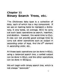
Since 2−1/c > 1/2, we conclude that the weight of vH is Θ(v) larger than the weight of v’s other child. The only way this difference in weight between the two children can occur is by insertions or deletion below v. Hence, Ω(v) updates must have been made below v since the last time v was involved in a partial rebuilding. In order for the amortized analysis to hold, we need to reserve a constant cost at v for each update below v. At each update, updates are made below O(log n) nodes, so the total reservation per update is O(log n). Since the tree is allowed to take any shape as long as its height is low enough, we call this type of balanced tree general balanced trees [7]. We use the notation GB-trees or GB(c)trees, where c is the height constant above. (The constant b is omitted in this notation.) (The idea of general balanced trees have also been rediscovered under the name scapegoat trees [33].) Example. The upper tree in Figure 10.5 illustrates a GB(1.2)-tree where five deletions and some insertions have been made since the last global rebuilding. When inserting 10, the height becomes 7, which is too high, since 7 > c log(|T |+d(T )) = 1.2 log(20+5) = 6. We back up along the path until we find the node 14. The height of this node is 5 and the weight is 8. Since 5 > 1.2 log 8, we can make a partial rebuilding at that node. The resulting tree is shown as the lower tree in Figure 10.5.

10.6.3

Application to Multi-Dimensional Search Trees

The technique of partial rebuilding is an attractive method in the sense that it is useful not only for ordinary binary search trees, but also for more complicated data structures, such as multi-dimensional search trees, where rotations cannot be used efficiently. For example, partial rebuilding can be used to maintain logarithmic height in k-d trees [19]

© 2005 by Chapman & Hall/CRC

Balanced Binary Search Trees

10-17

under updates [57, 68, 69]. A detailed study of the use of partial rebuilding can be found in Mark Overmars’ Ph.D. thesis [68]. For the sake of completeness, we just mention that if the
cost of rebalancing a subtree v is O(P (|v|)), the amortized cost of an update will  P (n) n

be O

log n . For example, applied to k-d trees, we get an amortized update cost of

2

O(log n).

10.7

Low Height Schemes

Most rebalancing schemes reproduce the result of AVL-trees [1] in the sense that they guarantee a height of c · log(n) for some constant c > 1, while doing updates in O(log n) time. Since the height determines the worst-case complexity of almost all operations, it may be reasonable to ask exactly how close to the best possible height log(n + 1) a tree can be maintained during updates. Presumably, the answer depends on the amount of rebalancing work we are willing to do, so more generally the question is: given a function f , what is the best possible height maintainable with O(f (n)) rebalancing work per update? This question is of practical interest—in situations where many more searches than updates are performed, lowering the height by factor of (say) two will improve overall performance, even if it is obtained at the cost of a larger update time. It is also of theoretical interest, since we are asking about the inherent complexity of maintaining a given height in binary search trees. In this section, we review the existing answers to the question. Already in 1976, Maurer et al. [55] proposed the k-neighbor trees, which guarantee a height of c · log(n), where c can be chosen arbitrarily close to one. These are unarybinary trees, with all leaves having the same depth and with the requirement that between any two unary nodes on the same level, at least k − 1 binary nodes appear. They may be viewed as a type of (1, 2)-trees where the rebalancing operations exchange children, not only with neighboring nodes (as in standard (a, b)-tree or B-tree rebalancing), but with nodes a horizontal distance k away. Since at each level, at most one out of k nodes is unary, the number of nodes increases by a factor of (2(k − 1) + 1)/k = 2 − 1/k for each level. This implies a height bound of log2−1/k n = log(n)/ log(2 − 1/k). By first order approximation, log(1 + x) = Θ(x) and 1/(1 + x) = 1 − Θ(x) for x close to zero, so 1/ log(2 − 1/k) = 1/(1 + log(1 − 1/2k)) = 1 + Θ(1/k). Hence, k-trees maintain a height of (1 + Θ(1/k)) log n in time O(k log n) per update. Another proposal [8] generalizes the red-black method of implementing (2, 4)-trees as binary trees, and uses it to implement (a, b)-trees as binary trees for a = 2k and b = 2k+1 . Each (a, b)-tree node is implemented as a binary tree of perfect balance. If the underlying (a, b)-tree has t levels, the binary tree has height at most t(k +1) and has at least (2k )t = 2kt nodes. Hence, log n ≥ tk, so the height is at most (k + 1)/k log n = (1 + 1/k) log n. As in red-black trees, a node splitting or fusion in the (a, b)-tree corresponds to a constant amount of recoloring. These operations may propagate along the search path, while the remaining rebalancing necessary takes place at a constant number of (a, b)-tree nodes. In the binary formulation, these operations involve rebuilding subtrees of size Θ(2k ) to perfect balance. Hence, the rebalancing cost is O(log(n)/k + 2k ) per update. Choosing k = log log n gives a tree with height bound log n + log(n)/ log log(n) and update time O(log n). Note that the constant for the leading term of the height bound is now one. To accommodate a non-constant k, the entire tree is rebuilt when log log n changes. Amortized this is O(1) work, which can be made a worst case bound by using incremental rebuilding [68]. Returning to k-trees, we may use the method of non-constant k also there. One possibility

© 2005 by Chapman & Hall/CRC

10-18

Handbook of Data Structures and Applications

is k = Θ(log n), which implies a height bound as low as log n + O(1), maintained with O(log2 n) rebalancing work per update. This height is O(1) from the best possible. A similar result can be achieved using the general balanced trees described in Section 10.6: In the proof of complexity in that section, the main point is that the cost |v| of a rebuilding at a node v can be attributed to at least (2−1/c − 1/2)|v| updates, implying that each update is attributed at most (1/(2−1/c − 1/2)) cost at each of the at most O(log n) nodes on the search path. The rebalancing cost is therefore O(1/(2−1/c − 1/2) log n) for maintaining height c · log n. Choosing c = 1 + 1/ log n gives a height bound of log n + O(1), maintained in O(log2 n) amortized rebalancing work per update, since (2−1/(1+1/ log n)) − 1/2) can be shown to be Θ(1/ log n) using the first order approximations 1/(1 + x) = 1 − Θ(x) and 2x = 1 + Θ(x) for x close to zero. We note that a binary tree with a height bound of log n + O(1) in a natural way can be embedded in an array of length O(n): Consider a tree T with a height bound of log n + k for an integer k, and consider n ranging over the interval [2i ; 2i+1 [ for an integer i. For n in this interval, the height of T never exceeds i + k, so we can think of T as embedded in a virtual binary tree T
with i + k completely full levels. Numbering nodes in T
by an in-order traversal and using these numbers as indexes in an array A of size 2i+k − 1 gives an embedding of T into A. The keys of T will appear in sorted order in A, but empty array entries may exist between keys. An insertion into T which violates the height bound corresponds to an insertion into the sorted array A at a non-empty position. If T is maintained by the algorithm based on general balanced trees, rebalancing due to the insertion consists of rebuilding some subtree in T to perfect balance, which in A corresponds to an even redistribution of the elements in some consecutive segment of the array. In particular, the redistribution ensures an empty position at the insertion point. In short, the tree rebalancing algorithm can be used as a maintenance algorithm for a sorted array of keys supporting insertions and deletions in amortized O(log2 n) time. The requirement is that the array is never filled to more than some fixed fraction of its capacity (the fraction is 1/2k−1 in the example above). Such an amortized O(log2 n) solution, phrased directly as a maintenance algorithm for sorted arrays, first appeared in [38]. By the converse of the embedding just described, [38] implies a rebalancing algorithm for low height trees with bounds as above. This algorithm is similar, but not identical, to the one arising from general balanced trees (the criteria for when to rebuild/redistribute are similar, but differ in the details). A solution to the sorted array maintenance problem with worst case O(log2 n) update time was given in [78]. Lower bounds for the problem appear in [28, 29], with one of the bounds stating that for algorithms using even redistribution of the elements in some consecutive segment of the array, O(log2 n) time is best possible when the array is filled up to some constant fraction of its capacity. We note that the correspondence between the tree formulation and the array formulation only holds when using partial rebuilding to rebalance the tree—only then is the cost of the redistribution the same in the two versions. In contrast, a rotation in the tree will shift entire subtrees up and down at constant cost, which in the array version entails cost proportional to the size of the subtrees. Thus, for pointer based implementation of trees, the above Ω(log2 n) lower bound does not hold, and better complexities can be hoped for. Indeed, for trees, the rebalancing cost can be reduced further. One method is by applying the idea of bucketing: The subtrees on the lowest Θ(log K) levels of the tree are changed into buckets holding Θ(K) keys. This size bound is maintained by treating the buckets as (a, b)-tree nodes, i.e., by bucket splitting, fusion, and sharing. Updates in the top tree only happen when a bucket is split or fused, which only happens for every Θ(K) updates in the bucket. Hence, the amortized update time for the top tree drops by a factor K. The buckets themselves can be implemented as well-balanced binary trees—using the schemes

© 2005 by Chapman & Hall/CRC

Balanced Binary Search Trees

10-19

above based on k-trees or general balanced trees for both top tree and buckets, we arrive at a height bound of log n + O(1), maintained with O(log log2 n) amortized rebalancing work. Applying the idea recursively inside the buckets will improve the time even further. This line of rebalancing schemes was developed in [3, 4, 9, 10, 42, 43], ending in a scheme [10] maintaining height log(n + 1) + 1 with O(1) amortized rebalancing work per update. This rather positive result is in contrast to an observation made in [42] about the cost of maintaining exact optimal height log(n + 1): When n = 2i − 1 for an integer i, there is only one possible tree of height log(n+ 1), namely a tree of i completely full levels. By the ordering of keys in a search tree, the keys of even rank are in the lowest level, and the keys of odd rank are in the remaining levels (where the rank of a key k is defined as the number of keys in the tree that are smaller than k). Inserting a new smallest key and removing the largest key leads to a tree of same size, but where all elements previously of odd rank now have even rank, and vice versa. If optimal height is maintained, all keys previously in the lowest level must now reside in the remaining levels, and vice versa—in other words, the entire tree must be rebuilt. Since the process can be repeated, we obtain a lower bound of Ω(n), even with respect to amortized complexity. Thus, we have the intriguing situation that a height bound of log(n+1) has amortized complexity Θ(n) per update, while raising the height bound a trifle to log(n + 1) + 1 reduces the complexity to Θ(1). Actually, the papers [3, 4, 9, 10, 42, 43] consider a more detailed height bound of the form log(n + 1) + ε, where ε is any real number greater than zero. For ε less than one, this expression is optimal for the first integers n above 2i − 1 for any i, and optimal plus one for the last integers before 2i+1 − 1. In other words, the smaller an ε, the closer to the next power of two is the height guaranteed to be optimal. Considering tangents to the graph of the logarithm function, it is easily seen that ε is proportional to the fraction of integers n for which the height is non-optimal. Hence, an even more detailed formulation of the question about height bound versus rebalancing work is the following: Given a function f , what is the smallest possible ε such that the height bound log(n + 1) + ε is maintainable with O(f (n)) rebalancing work per update? In the case of amortized complexity, the answer is known. In [30], a lower bound is given, stating that no algorithm using o(f (n)) amortized rebuilding work per update can guarantee a height of log(n + 1) + 1/f (n) for all n. The lower bound is proved by mapping trees to arrays and exploiting a fundamental lemma on density from [28]. In [31], a balancing scheme was given which maintains height log(n + 1) + 1/f (n) in amortized O(f (n)) time per update, thereby matching the lower bound. The basic idea of the balancing scheme is similar to k-trees, but a more intricate distribution of unary nodes is used. Combined, these results show that for amortized complexity, the answer to the question above is ε(n) ∈ Θ(1/f (n)). We may view this expression as describing the inherent amortized complexity of rebalancing a binary search tree, seen as a function of the height bound maintained. Using the observation above that for any i, log(n + 1) + ε is equal to log(n + 1) for n from 2i − 1 to (1 − Θ(ε))2i+1 , the result may alternatively be viewed as the cost of maintaining optimal height when n approaches the next power of two: for n = (1 − ε)2i+1 , the cost is Θ(1/ε). A graph depicting this cost appears in Figure 10.6. This result holds for the fully dynamic case, where one may keep the size at (1 − ε)2i+1 by alternating between insertions and deletions. In the semi-dynamic case where only insertions take place, the amortized cost is smaller—essentially, it is the integral of the function in Figure 10.6, which gives Θ(n log n) for n insertions, or Θ(log n) per insertion.

© 2005 by Chapman & Hall/CRC

Handbook of Data Structures and Applications Rebalancing Cost Per Update

10-20

60 50 40 30 20 10 0 0

10

20

30 40 Size of Tree

50

60

70

FIGURE 10.6: The cost of maintaining optimal height as a function of tree size.

More concretely, we may divide the insertions causing n to grow from 2i to 2i+1 into i segments, where segment one is the first 2i−1 insertions, segment two is the next 2i−2 insertions, and so forth. In segment j, we employ the rebalancing scheme from [31] with f (n) = Θ(2j ), which will keep optimal height in that segment. The total cost of insertions is O(2i ) inside each of the i segments, for a combined cost of O(i2i ), which is O(log n) amortized per insertion. By the same reasoning, the lower bound from [30] implies that this is best possible for maintaining optimal height in the semi-dynamic case. Considering worst case complexity for the fully dynamic case, the amortized lower bound stated above of course still applies. The best existing upper bound is height log(n + 1) +  min{1/ f (n), log(n)/f (n)}, maintained in O(f (n)) worst case time, by a combination of results in [4] and [30]. For the semi-dynamic case, a worst case cost of Θ(n) can be enforced when n reaches a power of two, as can be seen by the argument above on odd and even ranks of nodes in a completely full tree.

10.8

Relaxed Balance

In the classic search trees, including AVL-trees [1] and red-black trees [34], balancing is tightly coupled to updating. After an insertion or deletion, the updating procedure checks to see if the structural invariant is violated, and if it is, the problem is handled using the balancing operations before the next operation may be applied to the tree. This work is carried out in a bottom-up fashion by either solving the problem at its current location using rotations and/or adjustments of balance variables, or by carrying out a similar operation which moves the problem closer to the root, where, by design, all problems can be solved. In relaxed balancing, the tight coupling between updating and balancing is removed. Basically, any restriction on when rebalancing is carried out and how much is done at a time is removed, except that the smallest unit of rebalancing is typically one single or double rotation. The immediate disadvantage is of course that the logarithmic height guarantee disappears, unless other methods are used to monitor the tree height. The advantage gained is flexibility in the form of extra control over the combined process of updating and balancing. Balancing can be “turned off” during periods with frequent searching and updating (possibly from an external source). If there is not too much correlation between updates, the tree would likely remain fairly balanced during that time. When the frequency drops, more time can be spend on balancing. Furthermore, in multi-processor

© 2005 by Chapman & Hall/CRC

Balanced Binary Search Trees

10-21

environments, balancing immediately after an update is a problem because of the locking strategies with must be employed. Basically, the entire search path must be locked because it may be necessary to rebalance all the way back up to the root. This problem is discussed as early as in [34], where top-down balancing is suggested as a means of avoiding having to traverse the path again bottom-up after an update. However, this method generally leads to much more restructuring than necessary, up to Θ(log n) instead of O(1). Additionally, restructuring, especially in the form of a sequence of rotations, is generally significantly more time-consuming than adjustment of balance variables. Thus, it is worth considering alternative solutions to this concurrency control problem. The advantages outlined above are only fully obtained if balancing is still efficient. That is the challenge: to define balancing constraints which are flexible enough that updating without immediate rebalancing can be allowed, yet at the same time sufficiently constrained that balancing can be handled efficiently at any later time, even if path lengths are constantly super-logarithmic. The first partial result, dealing with insertions only, is from [41]. Below, we discuss the results which support insertion as well as deletion.

10.8.1

Red-Black Trees

In standard red-black trees, the balance constraints require that no two consecutive nodes are red and that for any node, every path to a leaf has the same number of black nodes. In the relaxed version, the first constraint is abandoned and the second is weakened in the following manner: Instead of a color variable, we use an integer variable, referred to as the weight of a node, in such a way that zero can be interpreted as red and one as black. The second constraint is then changed to saying that for any node, every path to a leaf has the same sum of weights. Thus, a standard red-black tree is also a relaxed tree; in fact, it is the ideal state of a relaxed tree. The work on red-black trees with relaxed balance was initiated in [64, 65]. Now, the updating operations must be defined so that an update can be performed in such a way that updating will leave the tree in a well-defined state, i.e., it must be a relaxed tree, without any subsequent rebalancing. This can be done as shown in Fig. 10.7. The operations are from [48]. The trees used here, and depicted in the figure, are assumed to be leaf-oriented. This terminology stems from applications where it is convenient to treat the external nodes differently from the remaining nodes. Thus, in these applications, the external nodes are not empty trees, but real nodes, possibly of another type than the internal nodes. In database applications, for instance, if a sequence of sorted data in the form of a linked list is already present, it is often desirable to build a tree on top of this data to facilitate faster searching. In such cases, it is often convenient to allow copies of keys from the leaves to also appear in the tree structure. To distinguish, we then refer to the key values in the leaves as keys, and refer to the key values in the tree structure as routers, since they merely guide the searching procedure. The ordering invariant is then relaxed, allowing keys in the left subtree of a tree rooted by u to be smaller than or equal to u.k, and the size of the tree is often defined as the number of leaves. When using the terminology outlined here, we refer to the trees as leaf-oriented trees. The balance problems in a relaxed tree can now be specified as the relations between balance variables which prevent the tree from being a standard red-black tree, i.e., consecutive red nodes (nodes of weight zero) and weights greater than one. Thus, the balancing scheme must be targeted at removing these problems. It is an important feature of the design that the global constraint on a standard red-black tree involving the number of black nodes is

© 2005 by Chapman & Hall/CRC

10-22

Handbook of Data Structures and Applications

FIGURE 10.7: Update operations.

not lost after an update. Instead, the information is captured in the second requirement and as soon as all weight greater than one has been removed, the standard constraint holds again. The strategy for the design of balancing operations is the same as for the classical search trees. Problems are removed if this is possible, and otherwise, the problem is moved closer to the root, where all problems can be resolved. In Fig. 10.8, examples are shown of how consecutive red nodes and weight greater than one can be eliminated, and in Fig. 10.9, examples are given of how these problems may be moved closer to the root, in the case where they cannot be eliminated immediately.

FIGURE 10.8: Example operations eliminating balance problems.

FIGURE 10.9: Example operations moving balance problems closer to the root.

It is possible to show complexity results for relaxed trees which are similar to the ones which can be obtained in the classical case. A logarithmic bound on the number of balancing operations required to balance the tree in response to an update was established in [23]. Since balancing operations can be delayed any amount of time, the usual notion of n as the number of elements in the tree at the time of balancing after an update is not really meaningful, so the bound is logarithmic in N , which is the maximum number of elements in the tree since it was last in balance. In [22], amortized constant bounds were obtained and in [45], a version is presented which has fewer and smaller operations, but meets the same bounds. Also, restructuring of the tree is worst-case constant per update. Finally, [48] extends the set of operations with a group insertion, such that an entire search tree

© 2005 by Chapman & Hall/CRC

Balanced Binary Search Trees

10-23

can be inserted in between two consecutive keys in amortized time O(log m), where m is the size of the subtree. The amortized bounds as well as the worst case bounds are obtained using potential function techniques [74]. For group insertion, the results further depend on the fact that trees with low total potential can build [40], such that the inserted subtree does not increase the potential too dramatically.

10.8.2

AVL-Trees

The first relaxed version of AVL-trees [1] is from [63]. Here, the standard balance constraint of requiring that the heights of any two subtrees differ by at most one is relaxed by introducing a slack parameter, referred to as a tag value. The tag value, tu , of any node u must be an integer greater than or equal to −1, except that the tag value of a leaf must be greater than or equal to zero. The constraint that heights may differ by at most one is then imposed on the relaxed height instead. The relaxed height rh(u) of a node u is defined as  tu , if u is a leaf rh(u) = max(rh(u.l), rh(u.r)) + 1 + tu , otherwise As for red-black trees, enough flexibility is introduced by this definition that updates can be made without immediate rebalancing while leaving the tree in a well-defined state. This can be done by adjusting tag values appropriately in the vicinity of the update location. A standard AVL-tree is the ideal state of a relaxed AVL-tree, which is obtained when all tag values are zero. Thus, a balancing scheme aiming at this is designed. In [44], it is shown that a scheme can be designed such that the complexities from the sequential case are met. Thus, only a logarithmic number of balancing operations must be carried out in response to an update before the tree is again in balance. As opposed to red-black trees, the amortized constant rebalancing result does not hold in full generality for AVL-trees, but only for the semi-dynamic case [58]. This result is matched in [46]. A different AVL-based version was treated in [71]. Here, rotations are only performed if the subtrees are balanced. Thus, violations of the balance constraints must be dealt with bottom-up. This is a minimalistic approach to relaxed balance. When a rebalancing operation is carried out at a given node, the children do not violate the balance constraints. This limits the possible cases, and is asymptotically as efficient as the structure described above [52, 53].

10.8.3

Multi-Way Trees

Multi-way trees are usually described either as (a, b)-trees or B-trees, which are treated in another chapter of this book. An (a, b)-tree [37, 57] consists of nodes with at least a and at most b children. Usually, it is required that a ≥ 2 to ensure logarithmic height, and in order to make the rebalancing scheme work, b must be at least 2a − 1. Searching and updating including rebalancing is O(log a n). If b ≥ 2a, then rebalancing becomes amortized O(1). The term B-trees [17] is often used synonymously, but sometimes refers to the variant where b = 2a − 1 or the variant where b = 2a. For (a, b)-trees, the standard balance constraints for requiring that the number of children of each node is between a and b and that every leaf is at the same depth are relaxed as follows. First, nodes are allowed to have fewer than a children. This makes it possible to perform a deletion without immediate rebalancing. Second, nodes are equipped with a tag value, which is a non-positive integer value, and leaves are only required to have the same

© 2005 by Chapman & Hall/CRC

10-24

Handbook of Data Structures and Applications

relaxed depth, which is the usual depth, except that all tag values encountered from the root to the node in question are added. With this relaxation, it becomes possible to perform an insertion locally and leave the tree in a well-defined state. Relaxed multi-way trees were first considered in [63], and complexity results matching the standard case were established in [50]. Variations with other properties can be found in [39]. Finally, a group insertion operation with a complexity of amortized O(loga m), where m is the size of the group, can be added while maintaining the already achieved complexities for the other operations [47, 49]. The amortized result is a little stronger than usual, where it is normally assumed that the initial structure is empty. Here, except for very small values of a and b, zero-potential trees of any size can be constructed such the amortized results starting from such a tree hold immediately [40].

10.8.4

Other Results

Even though there are significant differences between the results outlined above, it is possible to establish a more general result giving the requirements for when a balanced search tree scheme can be modified to give a relaxed version with corresponding complexity properties [51]. The main requirements are that rebalancing operations in the standard scheme must be local constant-sized operations which are applied bottom-up, but in addition, balancing operation must also move the problems of imbalance towards the root. See [35] for an example of how these general ideas are expressed in the concrete setting of red-black trees. In [32], it is demonstrated how the ideas of relaxed balance can be combined with methods from search trees of near-optimal height, and [39] contains complexity results made specifically for the reformulation of red-black trees in terms of layers based on black height from [67]. Finally, performance results from experiments with relaxed structures can be found in [21, 36].

References [1] G. M. Adel’son-Vel’ski˘ı and E. M. Landis. An algorithm for the organisation of information. Doklady Akadamii Nauk SSSR, 146:263–266, 1962. In Russian. English translation in Soviet Math. Doklady, 3:1259–1263, 1962. [2] A. V. Aho, J. E. Hopcroft, and J. D. Ullman. Data Structures and Algorithms. Addison-Wesley, Reading, Massachusetts, 1983. [3] A. Andersson. Optimal bounds on the dictionary problem. In Proceeding of the Symposium on Optimal Algorithms, volume 401 of Lecture Notes in Computer Science, pages 106–114. Springer-Verlag, 1989. [4] A. Andersson. Efficient Search Trees. PhD thesis, Department of Computer Science, Lund University, Sweden, 1990. [5] A. Andersson. Balanced search trees made simple. In Proceedings of the Third Workshop on Algorithms and Data Structures, volume 709 of Lecture Notes in Computer Science, pages 60–71. Springer-Verlag, 1993. [6] A. Andersson. A demonstration of balanced trees. Algorithm animation program (for macintosh) including user’s guide. Can be downloaded from author’s homepage, 1993. [7] A. Andersson. General balanced trees. Journal of Algorithms, 30:1–28, 1999. [8] A. Andersson, C. Icking, R. Klein, and T. Ottmann. Binary search trees of almost optimal height. Acta Informatica, 28:165–178, 1990. [9] A. Andersson and T. W. Lai. Fast updating of well-balanced trees. In Proceedings of

© 2005 by Chapman & Hall/CRC

Balanced Binary Search Trees

[10]

[11] [12] [13]

[14] [15] [16] [17] [18] [19] [20] [21]

[22]

[23] [24] [25] [26] [27] [28]

[29]

10-25

the Second Scandinavian Workshop on Algorithm Theory, volume 447 of Lecture Notes in Computer Science, pages 111–121. Springer-Verlag, 1990. A. Andersson and T. W. Lai. Comparison-efficient and write-optimal searching and sorting. In Proceedings of the Second International Symposium on Algorithms, volume 557 of Lecture Notes in Computer Science, pages 273–282. Springer-Verlag, 1991. A. Andersson and S. Nilsson. An efficient list implementation. In JavaOne Conference, 1999. Code can be found at Stefan Nilsson’s home page. Arne Andersson. A note on searching in a binary search tree. Software – Practice & Experience, 21(10):1125–1128, 1991. Arne A. Andersson and Mikkel Thorup. Tight(er) worst-case bounds on dynamic searching and priority queues. In Proceedings of the Thirty Second Annual ACM Symposium on Theory of Computing, pages 335–342. ACM Press, 2000. Lars Arge and Jeffrey Scott Vitter. Optimal external memory interval management. SIAM Journal on Computing, 32(6):1488–1508, 2003. R. Bayer. Binary B-trees for virtual memory. In Proceedings of the ACM SIGIFIDET Workshop on Data Description, Access and control, pages 219–235, 1971. R. Bayer. Symmetric binary B-trees: Data structure and maintenance algorithms. Acta Informatica, 1(4):290–306, 1972. R. Bayer and E. McCreight. Organization and maintenance of large ordered indexes. Acta Informatica, 1:173–189, 1972. Paul Beame and Faith E. Fich. Optimal bounds for the predecessor problem and related problems. Journal of Computer and System Sciences, 65(1):38–72, 2002. J. L. Bentley. Multidimensional binary search trees used for associative searching. Communications of the ACM, 18(9):509–517, 1975. N. Blum and K. Mehlhorn. On the average number of rebalancing operations in weight-balanced trees. Theoretical Computer Science, 11:303–320, 1980. Luc Boug´e, Joaquim Gabarr´ o, Xavier Messeguer, and Nicolas Schabanel. Concurrent rebalancing of AVL trees: A fine-grained approach. In Proceedings of the Third Annual European Conference on Parallel Processing, volume 1300 of Lecture Notes in Computer Science, pages 421–429. Springer-Verlag, 1997. Joan Boyar, Rolf Fagerberg, and Kim S. Larsen. Amortization results for chromatic search trees, with an application to priority queues. Journal of Computer and System Sciences, 55(3):504–521, 1997. Joan F. Boyar and Kim S. Larsen. Efficient rebalancing of chromatic search trees. Journal of Computer and System Sciences, 49(3):667–682, 1994. M. R. Brown. A storage scheme for height-balanced trees. Information Processing Letters, 7(5):231–232, 1978. M. R. Brown. Addendum to “A storage scheme for height-balanced trees”. Information Processing Letters, 8(3):154–156, 1979. H. Chang and S. S. Iynegar. Efficient algorithms to globally balance a binary search tree. Communications of the ACM, 27(7):695–702, 1984. A. C. Day. Balancing a binary tree. Computer Journal, 19(4):360–361, 1976. P. F. Dietz, J. I. Seiferas, and J. Zhang. A tight lower bound for on-line monotonic list labeling. In Proceedings of the Fourth Scandinavian Workshop on Algorithm Theory, volume 824 of Lecture Notes in Computer Science, pages 131–142. SpringerVerlag, 1994. P. F. Dietz and J. Zhang. Lower bounds for monotonic list labeling. In Proceedings of the Second Scandinavian Workshop on Algorithm Theory, volume 447 of Lecture Notes in Computer Science, pages 173–180. Springer-Verlag, 1990.

© 2005 by Chapman & Hall/CRC

10-26

Handbook of Data Structures and Applications

[30] Rolf Fagerberg. Binary search trees: How low can you go? In Proceedings of the Fifth Scandinavian Workshop on Algorithm Theory, volume 1097 of Lecture Notes in Computer Science, pages 428–439. Springer-Verlag, 1996. [31] Rolf Fagerberg. The complexity of rebalancing a binary search tree. In Proceedings of Foundations of Software Technology and Theoretical Computer Science, volume 1738 of Lecture Notes in Computer Science, pages 72–83. Springer-Verlag, 1999. [32] Rolf Fagerberg, Rune E. Jensen, and Kim S. Larsen. Search trees with relaxed balance and near-optimal height. In Proceedings of the Seventh International Workshop on Algorithms and Data Structures, volume 2125 of Lecture Notes in Computer Science, pages 414–425. Springer-Verlag, 2001. [33] I Galperin and R. L. Rivest. Scapegoat trees. In Proceedings of The Fourth Annual ACM-SIAM Symposium on Discrete Algorithms, pages 165–174, 1993. [34] Leo J. Guibas and Robert Sedgewick. A dichromatic framework for balanced trees. In

[35]

[36]

[37] [38]

[39]

[40]

[41] [42] [43]

[44]

[45] [46] [47]

Proceedings of the 19th Annual IEEE Symposium on the Foundations of Computer Science, pages 8–21, 1978. S. Hanke, Th. Ottmann, and E. Soisalon-Soininen. Relaxed balanced red-black trees. In Proceedings of the 3rd Italian Conference on Algorithms and Complexity, volume 1203 of Lecture Notes in Computer Science, pages 193–204. Springer-Verlag, 1997. Sabina Hanke. The performance of concurrent red-black tree algorithms. In Proceedings of the 3rd International Workshop on Algorithm Engineering, volume 1668 of Lecture Notes in Computer Science, pages 286–300. Springer-Verlag, 1999. Scott Huddleston and Kurt Mehlhorn. A new data structure for representing sorted lists. Acta Informatica, 17:157–184, 1982. Alon Itai, Alan G. Konheim, and Michael Rodeh. A sparse table implementation of priority queues. In Proceedings of the 8th International Colloquium on Automata, Languages and Programming, volume 115 of Lecture Notes in Computer Science, pages 417–431. Springer-Verlag, 1981. Lars Jacobsen and Kim S. Larsen. Complexity of layered binary search trees with relaxed balance. In Proceedings of the Seventh Italian Conference on Theoretical Computer Science, volume 2202 of Lecture Notes in Computer Science, pages 269– 284. Springer-Verlag, 2001. Lars Jacobsen, Kim S. Larsen, and Morten N. Nielsen. On the existence and construction of non-extreme (a, b)-trees. Information Processing Letters, 84(2):69–73, 2002. J. L. W. Kessels. On-the-fly optimization of data structures. Communications of the ACM, 26:895–901, 1983. T. Lai. Efficient Maintenance of Binary Search Trees. PhD thesis, Department of Computer Science, University of Waterloo, Canada., 1990. T. Lai and D. Wood. Updating almost complete trees or one level makes all the difference. In Proceedings of the Seventh Annual Symposium on Theoretical Aspects of Computer Science, volume 415 of Lecture Notes in Computer Science, pages 188– 194. Springer-Verlag, 1990. Kim S. Larsen. AVL trees with relaxed balance. In Proceedings of the 8th International Parallel Processing Symposium, pages 888–893. IEEE Computer Society Press, 1994. Kim S. Larsen. Amortized constant relaxed rebalancing using standard rotations. Acta Informatica, 35(10):859–874, 1998. Kim S. Larsen. AVL trees with relaxed balance. Journal of Computer and System Sciences, 61(3):508–522, 2000. Kim S. Larsen. Relaxed multi-way trees with group updates. In Proceedings of

© 2005 by Chapman & Hall/CRC

Balanced Binary Search Trees

[48] [49] [50] [51] [52] [53]

[54] [55] [56] [57] [58] [59]

[60] [61] [62] [63]

[64]

[65] [66] [67] [68] [69]

10-27

the Twentieth ACM SIGACT-SIGMOD-SIGART Symposium on Principles of Database Systems, pages 93–101. ACM Press, 2001. Kim S. Larsen. Relaxed red-black trees with group updates. Acta Informatica, 38(8):565–586, 2002. Kim S. Larsen. Relaxed multi-way trees with group updates. Journal of Computer and System Sciences, 66(4):657–670, 2003. Kim S. Larsen and Rolf Fagerberg. Efficient rebalancing of b-trees with relaxed balance. International Journal of Foundations of Computer Science, 7(2):169–186, 1996. Kim S. Larsen, Thomas Ottmann, and E. Soisalon-Soininen. Relaxed balance for search trees with local rebalancing. Acta Informatica, 37(10):743–763, 2001. Kim S. Larsen, E. Soisalon-Soininen, and Peter Widmayer. Relaxed balance using standard rotations. Algorithmica, 31(4):501–512, 2001. Kim S. Larsen, Eljas Soisalon-Soininen, and Peter Widmayer. Relaxed balance through standard rotations. In Proceedings of the Fifth International Workshop on Algorithms and Data Structures, volume 1272 of Lecture Notes in Computer Science, pages 450–461. Springer-Verlag, 1997. W. A. Martin and D. N. Ness. Optimizing binary trees grown with a sorting algorithm. Communications of the ACM, 15(2):88–93, 1972. H. A. Maurer, T. Ottmann, and H.-W. Six. Implementing dictionaries using binary trees of very small height. Information Processing Letters, 5:11–14, 1976. E. M. McCreight. Priority search trees. SIAM Journal on Computing, 14(2):257–276, 1985. Kurt Mehlhorn. Sorting and Searching, volume 1 of Data Structures and Algorithms. Springer-Verlag, 1986. Kurt Mehlhorn and Athanasios K. Tsakalidis. An amortized analysis of insertions into AVL-trees. SIAM Journal on Computing, 15(1):22–33, 1986. J. I. Munro. An implicit data structure for the dictionary problem that runs in polylog time. In Proceedings of the 25th Annual IEEE Symposium on the Foundations of Computer Science, pages 369–374, 1984. J. I. Munro. An implicit data structure supporting insertion, deletion and search in O(log2 n) time. Journal of Computer and System Sciences, 33:66–74, 1986. J. I. Munro and H. Suwanda. Implicit data structures for fast search and update. Journal of Computer and System Sciences, 21:236–250, 1980. J. Nievergelt and E. M. Reingold. Binary search trees of bounded balance. SIAM Journal on Computing, 2(1):33–43, 1973. O. Nurmi, E. Soisalon-Soininen, and D. Wood. Concurrency control in database structures with relaxed balance. In Proceedings of the 6th ACM Symposium on Principles of Database Systems, pages 170–176, 1987. Otto Nurmi and Eljas Soisalon-Soininen. Uncoupling updating and rebalancing in chromatic binary search trees. In Proceedings of the Tenth ACM SIGACT-SIGMODSIGART Symposium on Principles of Database Systems, pages 192–198, 1991. Otto Nurmi and Eljas Soisalon-Soininen. Chromatic binary search trees—a structure for concurrent rebalancing. Acta Informatica, 33(6):547–557, 1996. H. J. Olivie. A new class of balanced search trees: Half-balanced binary search trees. R. A. I. R. O. Informatique Theoretique, 16:51–71, 1982. Th. Ottmann and E. Soisalon-Soininen. Relaxed balancing made simple. Technical Report 71, Institut f¨ ur Informatik, Universit¨ at Freiburg, 1995. M. H. Overmars. The Design of Dynamic Data Structures, volume 156 of Lecture Notes in Computer Science. Springer-Verlag, 1983. Mark H. Overmars and Jan van Leeuwen. Dynamic multi-dimensional data structures

© 2005 by Chapman & Hall/CRC

10-28

Handbook of Data Structures and Applications

based on quad- and K -D trees. Acta Informatica, 17(3):267–285, 1982. [70] Daniel Dominic Sleator and Robert Endre Tarjan. Self-adjusting binary search trees. Journal of the ACM, 32(3):652–686, July 1985. [71] Eljas Soisalon-Soininen and Peter Widmayer. Relaxed balancing in search trees. In Advances in Algorithms, Languages, and Complexity, pages 267–283. Kluwer Academic Publishers, 1997. [72] Q. F. Stout and B. L. Warren. Tree rebalancing in optimal time and space. Communications of the ACM, 29(9):902–908, 1986. [73] R. E. Tarjan. Updating a balanced search tree in O(1) rotations. Information Processing Letters, 16:253–257, 1983. [74] Robert Endre Tarjan. Amortized computational complexity. SIAM Journal on Algebraic and Discrete Methods, 6(2):306–318, 1985. [75] Athanasios K. Tsakalidis. Rebalancing operations for deletions in AVL-trees. R.A.I.R.O. Informatique Th´eorique, 19(4):323–329, 1985. [76] J. van Leeuwen and M. H. Overmars. Stratified balanced search trees. Acta Informatica, 18:345–359, 1983. [77] M. A. Weiss. Data Structures and Algorithm Analysis. The Benjamin/Cummings Publishing Company, 1992. Several versions during the years since the first version. [78] Dan E. Willard. A density control algorithm for doing insertions and deletions in a sequentially ordered file in good worst-case time. Information and Computation, 97(2):150–204, 1992.

© 2005 by Chapman & Hall/CRC