DISSERTATION

Backscatter Radio Frequency Systems and Devices for Novel Wireless Sensing Applications

Conducted for the purpose of receiving the academic title “Doktorin der technischen Wissenschaften”

Submitted to Vienna University of Technology Faculty of Electrical Engineering and Information Technology

by

Dipl.-Ing. Jasmin Grosinger Fasangartengasse 6-8/4/6 1130 Wien Matriculation number: 9925521

Vienna, August 2012

Advisor Univ.Prof. Dipl.-Ing. Dr.techn. Arpad L. Scholtz Vienna University of Technology Institute of Telecommunications

Examiner Prof. Dr.-Ing. Dr.-Ing. habil. Robert Weigel University of Erlangen-N¨ urnberg Institute for Electronics Engineering

Acknowledgements It is a great pleasure to thank everyone who helped me write my dissertation successfully. First of all, I would like to show my deepest gratitude to my advisor, Professor Arpad L. Scholtz, for his encouragement, guidance, and support during the past four years. Furthermore, I am very grateful to Professor Robert Weigel for agreeing to review the thesis and to serve as examiner in my PhD thesis defense. I am truly indebted and thankful to Professor Christoph F. Mecklenbr¨auker, who supported me with his guidance and encouragement during the iTire project and throughout my PhD studies. Moreover, I would like to thank Joshua D. Griffin from Disney Research, Pittsburgh for giving me the opportunity to work with him on the backscatter bend sensor project. I am obliged to many of my colleagues who supported me, especially I am grateful for many fruitful discussions with Michael Fischer, Robert Langwieser, Gregor Lasser, and Lukas W. Mayer. I offer my regards to all of those who supported me in any respect during the completion of this dissertation. Finally, I owe sincere and earnest thankfulness to my family and my friends for there ever-present love and support.

Abstract This thesis examines the use of backscatter radio frequency identification (RFID) in novel wireless sensing applications. Backscatter RFID in sensor networks relies on the radio communication between an RFID reader, acting as a control unit, and a multitude of passive or semi-passive RFID transponders (tags), acting as sensor nodes. All power for the transmission of the sensor data is drawn from the electromagnetic field radiated by the reader. Hence, their low-power consumption makes backscatter tags appropriate for sensing applications that require small, light-weight, and low-maintenance sensor nodes. It is vital to ensure a reliable power transfer and wireless communication between the reader and the tags. Thus, the major design goal in this work is to realize backscatter RFID systems and devices which lead to high system performances. Particular attention is paid to the design of a tag antenna at 864 MHz for the wheel unit (WU) of an advanced tire monitoring system (ATMS). One premise of the application is that the antenna is directly attached to a car tire. The tire’s material parameters vary strongly with type and vendor of the tire. Thus, a tag antenna is prototyped which can cope with a change in the tire environment. An analysis shows that the antenna prototype assures a stable power supply to the tag’s chip for different tire environments and leads to a good system performance. In addition, an on-body backscatter RFID system is evaluated for remote health monitoring applications at 900 MHz and 2.45 GHz. The system performance is evaluated in a realistic indoor scenario through on-body channel measurements. An analysis of a state-of-the-art system example shows that the use of semi-passive chips leads to a reliable performance in the system’s forward link. A strategy to overcome limitations in the system’s backward link is to use a phase-modulated backscatter signal. Finally, a backscatter RFID sensor tag is designed that monitors the varying curvature of an object at 5.8 GHz. The backscatter sensor includes a transducer prototype which changes its impedance as a function of bending and directly modulates the carrier signal sent from the RFID reader. The transducer prototype is optimized with respect to the sensor’s sensitivity to bend and with respect to the sensor tag’s modulation efficiency. It is found that the prototype qualifies for integration in the sensor tag and assures a good RFID system performance.

i

Contents 1 Introduction 1.1 Backscatter RFID System . . . . . . . . . . . . . . . . . . . . 1.1.1 Backscatter Transponder . . . . . . . . . . . . . . . . . 1.1.2 Backscatter Radio Channel . . . . . . . . . . . . . . . 1.1.3 Interrogator . . . . . . . . . . . . . . . . . . . . . . . . 1.2 Scope of Work . . . . . . . . . . . . . . . . . . . . . . . . . . . 1.3 Outline and Related Work . . . . . . . . . . . . . . . . . . . . 1.3.1 Transponder Antenna for Car Tire Monitoring . . . . . 1.3.2 Communication System for Remote Health Monitoring 1.3.3 Sensor for Curvature Monitoring . . . . . . . . . . . . 2 Transponder Antenna for Car Tire Monitoring 2.1 Tire Environment . . . . . . . . . . . . . . . 2.1.1 Dielectric Properties of Tire Rubbers 2.1.2 Proximity Effects . . . . . . . . . . . 2.2 Antenna Prototype . . . . . . . . . . . . . . 2.2.1 Antenna Requirements . . . . . . . . 2.2.2 T-Matched Dipoles . . . . . . . . . . 2.3 Transponder Performance . . . . . . . . . . 2.3.1 Change in Tire Environments . . . . 2.3.2 Advanced Tire Monitoring System . 2.4 Summary . . . . . . . . . . . . . . . . . . .

. . . . . . . . .

. . . . . . . . .

. . . . . . . . .

1 2 2 9 10 13 13 13 14 15

. . . . . . . . . .

. . . . . . . . . .

. . . . . . . . . .

. . . . . . . . . .

. . . . . . . . . .

. . . . . . . . . .

. . . . . . . . . .

. . . . . . . . . .

. . . . . . . . . .

17 18 19 27 38 38 39 43 43 46 48

3 Communication System for Remote Health Monitoring 3.1 On-Body System . . . . . . . . . . . . . . . . . . . . 3.1.1 Body Model . . . . . . . . . . . . . . . . . . . 3.1.2 Antennas . . . . . . . . . . . . . . . . . . . . 3.2 Radio Channel . . . . . . . . . . . . . . . . . . . . . 3.2.1 Measurement Setup . . . . . . . . . . . . . . . 3.2.2 Comparison of Simulations and Measurements 3.2.3 Measurement Results . . . . . . . . . . . . . . 3.3 System Performance . . . . . . . . . . . . . . . . . . 3.3.1 Forward Link . . . . . . . . . . . . . . . . . . 3.3.2 Backward Link . . . . . . . . . . . . . . . . .

. . . . . . . . . .

. . . . . . . . . .

. . . . . . . . . .

. . . . . . . . . .

. . . . . . . . . .

. . . . . . . . . .

. . . . . . . . . .

. . . . . . . . . .

49 50 51 55 58 58 61 64 71 71 77

. . . . . . . . . .

. . . . . . . . . .

. . . . . . . . . .

. . . . . . . . . .

iii

3.4

Summary . . . . . . . . . . . . . . . . . . . . . . . . . . . . . . . .

4 Sensor for Curvature Monitoring 4.1 Sensing Approach . . . . . . . . . . . . 4.1.1 Antenna Transducer . . . . . . 4.1.2 Chip Transducer . . . . . . . . 4.2 Transducer Prototype . . . . . . . . . . 4.2.1 Microstrip Line Resonator . . . 4.2.2 Input Impedance Measurement 4.3 Sensor Performance . . . . . . . . . . . 4.4 Summary . . . . . . . . . . . . . . . . 5 Summary and Conclusions

iv

. . . . . . . .

. . . . . . . .

. . . . . . . .

. . . . . . . .

. . . . . . . .

. . . . . . . .

. . . . . . . .

. . . . . . . .

. . . . . . . .

. . . . . . . .

. . . . . . . .

. . . . . . . .

. . . . . . . .

. . . . . . . .

. . . . . . . .

81

83 . 84 . 84 . 85 . 92 . 92 . 93 . 95 . 100 101

1 Introduction Since the concept of modulating backscatter for communication was proposed in 1948 [1], considerable research and development has been invested in the area of backscatter radio frequency (RF) systems and devices, or rather backscatter radio frequency identification (RFID)1 systems and devices [2, 3]. Backscatter RFID in the ultra high frequency (UHF) and microwave frequency ranges is a promising communication technology for wireless sensing applications [4, 5]. In particular, the operation in the unlicensed frequency bands around 900 MHz [3], 2.45 GHz [3], and 5.8 GHz [6], is attractive for many sensor systems because of relatively large communication distances, comparatively small devices, and potentially high data rates. Backscatter RFID in sensor networks relies on the radio communication between an RFID reader, acting as a control unit, and a multitude of passive or semi-passive RFID transponders (tags), acting as sensor nodes. The principle of communication for transmitting information from the tag to the reader relies on a modulated backscatter signal. All power for the transmission of the sensor data is drawn from the electromagnetic field radiated by the reader. Hence, their low-power consumption makes backscatter tags appropriate for sensing applications that require small, light-weight, and low-maintenance nodes. In backscatter RFID systems, it is vital to ensure a reliable power transmission to the backscatter tags and to realize a robust wireless communication between the reader and tags. Thus, the proper design of backscatter RFID devices, which are included in sensor tags, and the investigation of backscatter radio channels are key study areas. This thesis examines the use of backscatter RFID in sensing applications like advanced tire monitoring, remote health monitoring, and curvature monitoring. Special attention is paid to prototyping and evaluation of backscatter RFID systems and devices, particularly to the development of systems and devices that are reliable in adverse operating environments like a car tire and the human body.

1

In general, the terms “backscatter RF” and “backscatter RFID” are used interchangeably in this work.

1

1 Introduction

Original Publications Related to This Chapter J. Grosinger, C. Mecklenbr¨auker, and A. Scholtz, “UHF RFID Transponder Chip and Antenna Impedance Measurements,” in Proc. International EURASIP Workshop on RFID Technology, September 2010. J. Grosinger and A. Scholtz, “Antennas and Wave Propagation in Novel Wireless Sensing Applications Based on Passive UHF RFID,” e&i Elektrotechnik und Informationstechnik, vol. 128, no. 11-12, pp. 408–414, 2011.

1.1 Backscatter RFID System A backscatter RFID system relies on the wireless communication between an RFID reader and a backscatter tag [3]. A schematic of the backscatter communication system with emphasis on the RFID tag is depicted in Fig. 1.1. The wireless communication link between the RFID reader and the backscatter tag can be divided into a forward link and a backward link. In the forward link, the RFID reader transmits RF power and data to the tag. In the backward link, whenever a reader command requires a tag’s response, the tag starts its data transfer using a modulated backscatter signal, i.e., the signal from the reader is reflected by the tag depending on the transmitted data. Typically, the reflected signal switches between two states and thus represent a logical ‘0’ and ‘1’.

1.1.1 Backscatter Transponder A conventional RFID tag consists of an antenna and an application specific integrated circuit chip. Fig. 1.1 shows such a tag. The tag’s antenna and chip are characterized by their complex impedances: by the impedance of the antenna, ZAnt = RAnt + XAnt and by the absorbing and reflecting impedances of the chip, ZAbs = RAbs + XAbs and ZRef = RRef + XRef . As stated earlier, the tag uses a modulated backscatter signal to communicate with the reader. Such a signal is realized by switching the chip’s input impedance between its absorbing impedance, ZAbs , and its reflecting impedance, ZRef (see Fig. 1.1). Hence, the signal from the reader is reflected at the chip’s input depending on the tag’s data. The reflected power at the chip’s input is related to reflection coefficients in the absorbing mode, SAbs , and the reflecting mode, SRef , which are defined by the antenna impedance and the respective chip impedance [7], SAbs =

2

∗ ∗ ZRef − ZAnt ZAbs − ZAnt and SRef = . ZAbs + ZAnt ZRef + ZAnt

(1.1)

1.1 Backscatter RFID System

RFID transponder

RFID reader Power and data

ZAnt ZAbs

ZRef

Modulated backscatter Chip Antenna

Figure 1.1: Backscatter RFID system with emphasis on the RFID tag: The backscatter tag consists of an antenna and a microchip which are characterized by their complex input impedances, ZAnt , ZAbs , and ZRef . In the case of an ideally amplitude-modulated backscatter signal2 , the reflection coefficient in the absorbing mode is zero, SAbs = 0 [3]. This is true for an impedance match between the antenna and the chip, i.e., the antenna’s impedance is the complex conjugate of the chip’s absorbing impedance [7], ∗ ZAnt = ZAbs .

(1.2)

As a consequence, the power available at the chip’s circuitry reaches its maximum. That is, the power transmission in the system’s forward link is maximized which corresponds to a power transmission coefficient of τ = 1 or rather τ = 100 %. This transmission coefficient is defined as [8, 9] τ = 1 − |SAbs |2 =

4RAbs RAnt . |ZAbs + ZAnt |2

(1.3)

The magnitude of the reflection coefficient in the reflecting state is one, |SRef | = 1, in the case of an ideally amplitude-modulated backscatter signal [3]. Consequently, the power in the backward link of the system is maximized. The modulation efficiency, η, compares the backscatter signal-relevant power reflected at the chip’s 2

In this work, an amplitude-modulated backscatter signal is assumed where not otherwise stated.

3

1 Introduction input with the available power at the antenna’s output and is defined as [9, 10] η=

2 2 4RAnt 2 · |ZAbs − ZRef |2 2 |S − S | = . Abs Ref π2 π 2 |ZAbs + ZAnt |2 · |ZRef + ZAnt |2

(1.4)

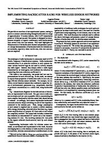
From Eqn. 1.4, it follows that a modulation efficiency of η ≈ 20 % can be achieved for an ideally amplitude-modulated backscatter signal, i.e., SAbs = 0 and |SRef | = 1. A maximum modulation efficiency of π82 ≈ 81 % can be realized for reflection coefficients which have magnitudes of 1 and contrary phases [10], i.e., for an ideally phase-modulated backscatter signal with SAbs = 1 and SRef = −1 [3]. Transponder Chip In general, an off-the-shelf RFID chip is a nonlinear load whose complex impedance in each state varies with the frequency and input power. The power dependence is determined by the details of the chip’s RF frontend and the power consumption of the specific chip, while the frequency dependence is mostly due to the chip’s parasitic and packaging effects [11]. To maximize the power transfer in the forward and backward links of a backscatter system, knowledge of the chip’s impedances is mandatory. As an example, Fig. 1.2 plots the measured impedance in the absorbing mode, ZAbs , of a passive UHF RFID chip at a frequency of f = 864 MHz. The knowledge of ZAbs is especially important in the case of a passive RFID chip which does not have its own power supply and thus relies completely on the wireless power transfer from the reader. In Fig. 1.2, the absorbing impedance of the exemplary chip, ZAbs = RAbs + XAbs , is plotted versus the chip’s input power, PTag . It can be seen that ZAbs is highly reactive. Additionally, the impedance changes drastically at high power levels. This is due to an internal power regulation in the chip, the absorbing impedance converges with increasing power to the reflecting impedance to protect the chip’s internal circuit [9]. A backscatter tag chip needs a certain minimum power to turn on its circuitry. This power level is known as the chip’s sensitivity, TChip . Again, this threshold is defined by the details of the chip’s RF frontend. The chip’s sensitivity, TChip , can be found by measuring the chip’s input impedances versus its input power [9]. Offthe-shelf passive RFID chips, which do not have their own power supply, have chip sensitivities of about −15 dBm, e.g., TChip = −17.8 dBm [12], while semi-passive chips feature sensitivities down to −40 dBm [13]. Semi-passive chips have their own power supply to activate the chip’s circuitry. Additionally, they harvest power and use power-saving backscattering for the communication with the reader [14].

4

1.1 Backscatter RFID System

300 RAbs

200

XAbs

RAbs , XAbs (Ω)

100 0 −100 −200 −300 −400 −500 −30

−25

−20

−15

−10 PTag (dBm)

−5

0

5

9

Figure 1.2: Absorbing impedance of an exemplary chip, ZAbs = RAbs +XAbs , versus the chip’s input power, PTag , at 864 MHz Transponder Antenna Proper impedance matching between the tag’s antenna and the chip is very important for backscatter RFID systems. Typically, the input impedance of the chip cannot be chosen arbitrarily due to technological limits. Thus, the antenna’s impedance is optimized to match the chip’s impedance. As stated earlier, knowledge of the chip’s absorbing impedance allows a tag antenna design which is optimized to maximize the forward link of the backscatter RFID system. This impedance matching is usually done at the chip’s sensitivity, TChip [15]. In the example presented above (see Fig. 1.2), the absorbing impedance is ZAbs = (68 − 442) Ω. Fig. 1.3 plots the power transmission coefficient, τ , versus the antenna’s impedance, ZAnt (see Eqn. 1.3). It can be seen that τ is indeed maximized for an antenna impedance of ZAnt = (68 + 442) Ω as stated in Eqn. 1.2. In addition, the antenna impedance can be optimized to maximize the signal that is reradiated towards the reader which is equivalent to the use of a phase-modulated backscatter signal. For this optimization, the knowledge of both chip impedances is mandatory [9], s ZAnt =

RAbs RRef

(RAbs + RRef )2 + (XAbs − XRef )2 RRef XAbs + RAbs XRef − . 2 (RAbs + RRef ) RAbs + RRef (1.5)

5

1 Introduction In Fig. 1.4, the modulation efficiency, η, is plotted versus the antenna’s impedance, ZAnt , for an absorbing impedance of ZAbs = (68 − 442) Ω and a reflecting impedance of ZRef = (2 − 0.1) Ω (see Eqn. 1.4). η reaches its maximum for an antenna impedance of ZAnt = (75 + 13) Ω, while the power transmission coefficient is modest 10 % (see Fig. 1.3). Thus, such an optimization is only advisable if the forward link can tolerate small power transmission coefficients. For an antenna impedance of ZAnt = (68 + 442) Ω, η is 20 % according to Eqn. 1.4 for SAbs = 0 and |SRef | = 1. The variation of the chip’s impedances as a result of the input power can drastically affect the matching between the tag’s antenna and chip. It is possible to have a situation where a significant variation of the chip’s impedances results in dead spots within the operational range of the tag [16]. Today’s backscatter RFID systems combat this effect by using for example transmit diversity at the RFID reader [17]. Scattering Properties of Antennas In general, the power reflected from a receiving antenna for any load impedance can be written as the sum of two terms [18], the power scattered due to the antenna mode and the power scattered due to the structural mode of the antenna [9]. Consequently, it is incorrect to assume that the receiving antenna scatters as much ∗ as its absorbs under matched load conditions [19], i.e., ZAnt = ZAbs . In general, the reflected power may be larger, equal to, or smaller than the absorbed power [19]. The reflected power due to the antenna mode depends on the chip’s impedances, while the power due to the antenna’s structural mode is not influenced by an impedance change. Thus, the structural scattering component cannot be used for the data transmission in an RFID system and is not relevant for RFID applications [9]. This scattering component is similar to a reflected signal that is caused by an interacting object in the propagation path between the reader and tag and is furthermore treated as such (see Sec. 1.1.3).

6

1.1 Backscatter RFID System

500 80 % 90 %

400

70 %

60 % 50 % 40 %

300

20 %

XAnt (Ω)

200

100 30 %

0

10 %

−100

−200

0

50

100

150

200

250 300 RAnt (Ω)

350

400

450

500

Figure 1.3: Power transmission coefficient, τ , versus the antenna’s impedance, ZAnt = RAnt + XAnt , for ZAbs = (68 − 442) Ω: The optimized antenna impedances, ZAbs = (68 − 442) Ω according to Eqn. 1.2 and ZAnt = (75 + 13) Ω according to Eqn. 1.5, are highlighted.

7

1 Introduction

500 30 %

400 30 % 40 % 20 %

300

XAnt (Ω)

200

60 %

100

70 %

0

50 %

−100

10 %

20 %

−200

0

50

100

150

200

250 300 RAnt (Ω)

350

400

450

500

Figure 1.4: Modulation efficiency, η, versus the antenna’s impedance, ZAnt = RAnt + XAnt , for ZAbs = (68 − 442) Ω and ZRef = (2 − 0.1) Ω: The optimized antenna impedances, ZAbs = (68 − 442) Ω according to Eqn. 1.2 and ZAnt = (75 + 13) Ω according to Eqn. 1.5, are highlighted.

8

1.1 Backscatter RFID System

1.1.2 Backscatter Radio Channel In a backscatter RFID system, a bidirectional radio link is established between the reader and tag — the reader-tag-reader link — which can be subclassified into the forward link and backward link [6]. The link budget of the backscatter radio channel is outlined in Fig. 1.5. In the forward link, the reader transmits RF power, PTX,Reader , and data to the tag. The power absorbed by the tag’s chip, PChip , is defined by [9] PChip = τ PTag = τ |S21 |2 PTX,Reader ,

(1.6)

where PTag is the chip’s input power and S21 is the channel transfer function of the forward link. PChip should be higher than the chip’s sensitivity, TChip . If PChip is smaller than TChip , the backscatter communication is limited in its forward link [16]. In the backward link, the tag responds to the reader by modulating the backscattered signal. The power of the tag’s signal at the receiver (RX) of the reader, PRX,Reader , can be written as [9] PRX,Reader = |S12 |2 ηPChip = |S12 |2 η|S21 |2 PTX,Reader ,

(1.7)

where S12 is the channel transfer function of the backward link. PRX,Reader should be higher than the RX’s sensitivity, TRX,Reader , which is defined as the minimum input power at the reader to assure a successful reception of the tag’s data. If PRX,Reader is smaller than TRX,Reader , the communication system is limited in its backward link [16]. The channel transfer functions, S21 and S12 , depend on the antenna characteristics of the reader and tag (e.g., antenna gain, polarization) and the properties of the propagation channel (e.g., path loss, fading) [20].

9

1 Introduction

RFID transponder

RFID reader

PTX,Reader

|S21 |2 PTag PChip = τ PTag ηPTag

PRX,Reader |S12 |2 Ref

Figure 1.5: Link budget of the backscatter radio channel

1.1.3 Interrogator Fig. 1.6 depicts the RF architecture of an RFID reader with a monostatic antenna configuration [11]. Such a configuration applies a single antenna for the transmit and receive paths which are — in this example — separated by a circulator. The transmitter (TX) produces the RF signal to power the tag and to send commands, while the RX takes care of amplifying and purifying the received signal [21]. A baseband processor generates the command sequences, demodulates the received signals, and controls the protocol. The reader constantly transmits a continuous wave signal to the tag except during the times of interrogation when the carrier is modulated. After a certain idle period, the tag responds to the reader by backscattering the carrier [22]. During the entire process, the transmit signal leaks into the receive path. The amplitude of the leakage signal depends on the TX to RX decoupling concept [23]. Here, the amplitude of the leakage depends on the isolation of the circulator and the antenna matching. In addition, the leakage signal includes scattered signal components from static scatterers in the propagation environment as well as static reflections due to the tag antenna’s structural mode and antenna mode (see Sec. 1.1.1). In a practical system, the carrier leakage can be 65 dB to 90 dB stronger than the backscattered signal [23], making it necessary to estimate its extent and subtract it from the received signal, e.g., by the use of a carrier compensation unit [24].

10

1.1 Backscatter RFID System

Transmitter

Circulator Baseband processor

Antenna

Receiver

Figure 1.6: RFID reader with a monostatic antenna configuration [11] Baseband Signal Constellations at the Reader Receiver At the RX part of the baseband processor, the received signal is downconverted to the baseband. Fig. 1.7 shows an exemplary signal constellation in the baseband’s inphase (I) and quadrature (Q) plane of the reader RX [23]. If the tag is absorbing energy, the reader finds the tag’s absorb state in its I/Q plane, S (A) , which is essentially the carrier leakage, L [23]. If the tag starts to transmit information to the reader, the reader encounters the tag’s reflect state, S (R) . The tag’s signal, h, adds up with the carrier leakage, L + h [23]. h depends on the channel transfer functions, S21 and S12 , and on the modulation behavior of the tag which is determined by SAbs and SRef [23]. Digital reader RX architectures are capable of estimating the two states, S (A) and S (R) , by employing a carrier cancelation and a channel estimation [23]. Such RXs feature sophisticated detection algorithms at the reader and allow for example the detection of multiple tags during a collision [23].

11

1 Introduction

Quadrature

S (A) Carrier leakage L

Tag signal h

h S (R)

Inphase

Figure 1.7: Exemplary baseband constellation at the RFID reader RX [23]

12

1.2 Scope of Work

1.2 Scope of Work This thesis examines the use of backscatter RFID systems in novel wireless sensing applications. Particular attention is paid to the tag antenna design of a wheel unit (WU) in an advanced tire monitoring system (ATMS), the performance of an onbody RFID system for a wireless body area network (WBAN), and the design of a transducer for a backscatter bend sensor to monitor the curvature of an object. As stated earlier, it is vital to ensure a reliable power transfer and wireless communication between the reader and the tag. For example, if the power at the tag’s chip is smaller than the chip’s sensitivity, the backscatter communication system is limited in its forward link. If the power at the reader RX is smaller than the RX’s sensitivity, a limitation in the backward link occurs. Thus, the major design goal in this work is to realize backscatter RFID systems and devices which lead to high system performances. Special care is taken to realize systems and devices which operate efficiently in a car tire and on the human body whereas in the case of the backscatter sensor, the focus is on low power consumption and an acceptable sensitivity to bend.

1.3 Outline and Related Work The main contributions of this thesis comprised in Chap. 2, Chap. 3, and Chap. 4 are briefly summarized in this section.

1.3.1 Transponder Antenna for Car Tire Monitoring Chap. 2 deals with the design of a tag antenna at 864 MHz for the WU of an ATMS based on backscatter RFID. One premise of the application is that the antenna is directly attached to a car tire. Thus, the antenna’s surroundings and proximity effects caused by the tire environment are explored. Measurements of the dielectric properties of the tire rubber show that the material parameters vary strongly with type and vendor of the tire. This fact leads to a detuning of the WU antenna which is rather difficult to predict. Consequently, a tag antenna is prototyped which can cope with a change in the tire environment. The prototype is power-matched to the tag’s chip over a wide range of frequencies. Further analyses show that the antenna prototype assures a stable power supply to the tag’s chip and leads to a good performance in an ATMS based on passive UHF RFID. In addition, another proximity effect due to the car tire — the distortion of the antenna’s radiation pattern — is beneficially exploited and leads to a further enhancement in the tag’s performance.

13

1 Introduction Related Work Previous research has focused on the design of WU antennas for classical tire pressure monitoring systems (TPMSs) without the use of backscatter RFID. For example, Brzeska et al. [25] studies and characterizes a WU with an integrated antenna mounted on the valve of a car tire at 434 MHz. Investigations of a small loop antenna operating at 315 MHz, which is mounted on the rim of a car tire, are presented by Tanoshita et al. [26], while Teranishi et al. [27] provides simulations of a helical WU antenna mounted on the rim of a truck tire. Car tire monitoring based on a backscatter RFID system has received less attention in the literature. Lasser and Mecklenbr¨auker [28, 29] characterize the propagation channel of an ATMS at 868 MHz and 2.45 GHz. A detailed investigation of such a system in terms of its backscatter performance in the forward link using dual-antenna WU RFID tags is done by Lasser et al. [30]. Basat et al. [31] present passive RFID tag antennas at 915 MHz which are designed for inventory purposes of car tires. Peyerl [32] investigates in his diploma thesis tire structures and characterizes the material properties of tire rubbers at UHFs for the purpose of a proper tag antenna design.

1.3.2 Communication System for Remote Health Monitoring Chap. 3 investigates an on-body backscatter RFID system for remote health monitoring applications in the UHF range at 900 MHz and 2.45 GHz. The investigation is done for two different on-body antenna types. Monopole antennas act as a best-case reference, while less efficient patch antennas are used to give insight into practical RFID system implementations. The antennas are designed by means of a body model to account for proximity effects that are caused by human tissue. The system performance is evaluated in a realistic indoor scenario through on-body channel measurements. The evaluation provides outage probabilities for the system’s forward and backward links. These probabilities help to identify limitations in the backscatter system and to evaluate strategies to overcome these barriers for the realization of a reliable on-body RFID system. An analysis of a state-of-the-art system example shows that the use of semi-passive chips leads to a reliable performance in the system’s forward link. A strategy to overcome limitations in the system’s backward link is to use a phase-modulated backscatter signal. Related Work Previous studies on UHF RFID based WBANs have focused on in-body and offbody communication systems. This classification of WBANs has been introduced by Hall and Hao [33]. For example, Occhiuzzi et al. [34] investigate backscatter sensor tags implanted in the human body and their communication to an external reader for vascular

14

1.3 Outline and Related Work monitoring applications. Sani et al. [35] compare passive and active RFID tags implanted in the human body for tracking and identification purposes, while Schmidt et al. [36] concentrate on the antenna design of implanted RFID tags. RFID sensor tags which are mounted on the human body for the monitoring of sleep diseases are explored by Occhiuzzi et al. [37]. Backscatter identification of people based on on-body backscatter tags is the driving force behind the research of Polivka et al. [38]. Cotton et al. [39] explore the backscatter communication links between an active, wrist-worn tag and four readers in an indoor environment. Onbody tag antenna designs for identification and tracking applications are presented by Kellom¨aki et al. [40], by Rajagopalan and Rahmat-Samii [41], and by Ziai and Batchelor [42]. So far, the investigation of backscatter communication systems on the human body has received less attention in the literature. A first feasibility study of onbody backscatter RFID systems is presented by Manzari et al. [43, 44] and is based on a backscatter measurement at 870 MHz. The RFID system consists of a short range reader composed of a patch antenna and five on-body tags consisting of custom-built wearable felt antennas.

1.3.3 Sensor for Curvature Monitoring Chap. 4 provides a design for a backscatter RFID sensor tag that monitors the varying curvature of an object at 5.8 GHz. The backscatter sensor includes a transducer, which changes its impedance as a function of bending, in the tag antenna’s load and thus directly modulates the carrier signal sent from the RFID reader. In addition, the transducer, which acts as the chip’s reflecting impedance, assures a stable power supply to the chip’s circuitry and benefits the detection at the RFID reader. A microstrip line resonator is prototyped for integration in such a backscatter bend sensor. The resonator’s backscatter transducer efficiency is evaluated and optimized with respect to the sensor’s sensitivity to bend and with respect to the sensor tag’s modulation efficiency. It is found that the prototype qualifies for integration in the sensor tag and assures a good RFID system performance. Related Work Previous research on the integration of sensing abilities in backscatter RFID tags, without the use of additional RF circuitry, has focused on the use of antenna transducers, i.e., the tag’s antenna acts as the transducer. For example, Capdevila et al. [45] present the use of passive RFID tags for continuous monitoring of the water temperature and discrete monitoring of liquid levels. Bhattacharyya et al. [46] present tag antenna-based sensing of temperature thresholds, displacements, and liquid levels. Siden et al. [47] present another antenna transducer which is used to sense the moisture content in walls. Caizzone et al. [48] realize an antenna trans-

15

1 Introduction ducer by using a shape memory alloy as part of the tag’s antenna to detect a temperature threshold violation. An approach to realize an antenna transducer design for gas detection using single-walled carbon nanotubes (SWCNTs) is presented by Occhiuzzi et al. [49]. The chip transducer approach has received less attention in the literature. Tentzeris and Nikolaou [50] present a chip transducer design for a chipless RFID tag which uses a film of SWCNTs as the antenna load to detect toxic gas. Another chipless RFID tag to sense gas is presented by Balachandran et al. [51, 52].

16

2 Transponder Antenna for Car Tire Monitoring Car tire monitoring is an important safety feature in modern vehicles and strongly improves the reliability of tires and tire control systems [53, 54]. As a consequence, a lot of effort is put into the development of ATMSs which upgrade conventional TPMSs [55] by additionally acquiring sensor data like tire temperature, contact area, vertical load, slip angle, and street conditions. An ATMS is composed of sensor nodes — WUs — mounted in each tire and a control unit — the on-board unit (OU) — located in the car body. Backscatter RFID in the UHF range around 900 MHz is a promising communication technology to power up the WUs, read out the sensor data, and support lifecycle management and identification of the tires. In conventional TPMSs, the WU and its antenna is integrated into the valve or is mounted on the rim of the wheel. In ATMSs, the WU must directly contact the tire tread to enable the measurement of additional sensor data. Thus, one of the challenges in realizing backscatter UHF RFID in an ATMS is the design of efficient tag antennas which are directly attached to the tires. An antenna in the complex environment of a car tire will be influenced by this surroundings. This chapter deals with the design of a tag antenna for a WU of an ATMS based on backscatter RFID at 864 MHz. Sec. 2.1 explores the antenna’s environment as well as the proximity effects caused by the tire. In Sec. 2.2, the tag antenna’s requirements are listed and an appropriate antenna prototype is designed. Sec. 2.3 analyzes the tag’s performance in terms of varying tire environments and the system’s forward link using a passive tag.

Original Publications Related to This Chapter J. Grosinger, L. Mayer, C. Mecklenbr¨auker, and A. Scholtz, “Antenna Design for a Car Tire,” in Proc. Radar, Communication and Measurement, March 2009. J. Grosinger, L. Mayer, C. Mecklenbr¨auker, and A. Scholtz, “Determining the Dielectric Properties of a Car Tire for an Advanced Tire Monitoring System,” in Proc. Vehicular Technology Conference, September 2009.

17

2 Car Tire Monitoring J. Grosinger, L. Mayer, C. Mecklenbr¨auker, and A. Scholtz, “Input Impedance Measurement of a Dipole Antenna Mounted on a Car Tire,” in Proc. International Symposium on Antennas and Propagation, October 2009. J. Grosinger, C. Mecklenbr¨auker, and A. Scholtz, “Design Considerations for UHF Antennas Deployed Inside Car Tires,” in Proc. Electrical and Electronic Engineering for Communication, June 2010. J. Grosinger, G. Lasser, C. Mecklenbr¨auker, and A. Scholtz, “Gain and Efficiency Measurement of Antennas for an Advanced Tire Monitoring System,” in Proc. IEEE International Symposium on Antennas and Propagation and CNC/USNC/URSI Radio Science Meeting, July 2010. J. Grosinger, C. Mecklenbr¨auker, and A. Scholtz, “UHF RFID Transponder Chip and Antenna Impedance Measurements,” in Proc. International EURASIP Workshop on RFID Technology, September 2010. J. Grosinger and M. Fischer, “Bandwidth Issues of UHF RFID Transponder Antennas for Advanced Tire Monitoring,” in Proc. IEEE-APS Topical Conference on Antennas and Propagation in Wireless Communications, September 2011. J. Grosinger and A. Scholtz, “Antennas and Wave Propagation in Novel Wireless Sensing Applications Based on Passive UHF RFID,” e&i Elektrotechnik und Informationstechnik, vol. 128, no. 11-12, pp. 408–414, 2011. G. Lasser, J. Grosinger, R. Langwieser, and C. Mecklenbr¨auker, “Measurement Based Performance Evaluation of Advanced Tire Monitoring Systems Using RFID Technology,” in Proc. IEEE International Microwave Symposium, June 2012. Workshop Presentation.

2.1 Tire Environment It is important to have a thorough knowledge of the tire’s structure and its material properties to evaluate the influence of the tire on the tag antenna. Thus, the structure of a modern radial car tire is investigated. Its construction is shown in Fig. 2.1. The tire is composed of multiple rubber layers as well as metal and fiber reinforcements. These components ensure the main functions of the tire: load carrying and transfer of acceleration, deceleration, and lateral forces [56]. From an RF point of view, the tire can be divided into two sections, the tire sidewalls and the tire tread [25]. The sidewalls are composed of different rubber layers, a carcass which is mainly composed of fiber reinforcements, and tire beads with steel cores to anchor the tire on a rim. In contrast, the tread includes different rubber layers, the carcass, and a steel belt. The steel belt is made of two parallel layers of steel wires, in each layer the wires draw an angle of plus and minus 25 ◦ (depending on the tire type) with respect to the direction of motion.

18

2.1 Tire Environment

Tread Sidewall Steel belt Carcass

Bead with steel core

Figure 2.1: Construction of a modern radial car tire: complex structure with multiple rubber layers, metal and fiber reinforcements [57]

2.1.1 Dielectric Properties of Tire Rubbers The different rubber layers of the tire can be considered as lossy dielectrics. A dielectric material is characterized by a complex relative permittivity [58], ε˜r = εr − jε00r ,

(2.1)

at a certain frequency. In the dielectric material, the arrangement of constituent atoms and molecules, i.e., the orientation of their charges, is changed as a reaction to an external electric field. A measure of the amount of polarization that occurs for the applied field is the relative permittivity, εr . ε00r is a measure of the losses in the material due to the friction associated with the changing polarization and the drift of conduction charges. The loss tangent, tan(δ), is defined as [58] tan(δ) =

ε00r , εr

(2.2)

and characterizes the relative loss in the dielectric, which is the ratio of the energy lost and the energy stored within one cycle of the RF field. Open-Ended Coaxial Probe Technique The dielectric properties of each rubber layer of the tire are measured by means of an open-ended coaxial probe technique. Here, an open-ended coaxial probe is

19

2 Car Tire Monitoring pressed against the rubber under test (RUT). The field of the probe fringes into the dielectric material and is measured by means of a vector network analyzer (VNA). The measured reflection coefficient, S11 , at the end of the coaxial probe leads to the RUT’s material parameters [59]. The open-ended coaxial probe technique is a broadband testing method [60] and is non-destructive in the sense that it does not require a specimen to be shaped to fit a particular sample holder geometry. This is an advantage in the case of the care tire because the different rubber layers of the tire are difficult to separate. To perform the method, the following preconditions must be fulfilled [61]: • The surface of the material has to be flat. Thus, a piece of the tire is cut out and polished to obtain a flat surface (see Fig. 2.7). • The material has to have semi-infinite thickness. This means that the rubber sample must be thick enough to appear infinite to the probe’s field. A simple practical approach to verify this requirement is to check if the measurement results are affected by the presence of metal at the material’s perimeter [61]. • Another precondition is that there must not be air gaps between the probe and the RUT. Thus, the probe is fixed in a micromanipulator (see Fig. 2.2) and carefully pressed against the RUT till a stable measurement result is realized. • The RUT has to be non-magnetic. It is assumed that the magnetic response of the tire rubber is very weak and thus negligible. • The RUT has to be homogenous and isotropic. The RUT is assumed to be linear, homogenous, and isotropic. The measurement setup with the micromanipulator, the coaxial probe, and the tire specimen can be seen in Fig. 2.2. The reflection coefficient, S11 , is measured at room temperature with Rohde&Schwarz’s ZVA24 VNA versus a frequency range of 100 MHz − 5 GHz. The VNA is connected to the 50 Ω coaxial probe via a test cable and is calibrated by means of short, open, and matched load standards, while the electrical length of the coaxial probe is de-embedded by means of an electrical short [62]. There are two basic approaches to derive the complex relative permittivity, ε˜r , from the measurement results [63]. The first approach uses an equivalent circuit of the probe’s fringing field [59]. The second approach calculates the probe’s field by numerically solving Maxwell’s equations [64]. Here, the latter one is used which leads to the benefit that no reference materials are needed [59]. In particular, ε˜r is obtained by solving the electromagnetic field using Ansys’ HFSS [65]. An HFSS model is designed which is practically equivalent to the measurement setup. The model is shown in Fig. 2.3. The coaxial probe is composed of an inner conductor with a radius of 0.65 mm, a Teflon substrate with a thickness of

20

2.1 Tire Environment

Open-ended coaxial probe VNA cable

Tire specimen

Micromanipulator

Figure 2.2: Measurement setup: micromanipulator with micrometer screw, VNA test cable, open-ended coaxial probe, and tire specimen 1.35 mm, and an outer conductor with a thickness of 0.35 mm. The RUT is modeled as a cylinder with a radius and a height of 10 mm. Simulations show that these dimensions are large enough to contain the fringing field in the dielectric. The material’s dielectric properties are defined by εr and tan(δ). A wave port is used to excite the structure. The blue arrow in Fig. 2.3 denotes the de-embedding of the port to the end of the coaxial probe. As with the measurement, the port impedance is 50 Ω. In addition, an air box surrounds the whole simulation setup to avoid perfectly conducting boundaries at the tire material [66]. The effect of the RUT’s material parameters on the reflection coefficient is illustrated in Fig. 2.4 by means of simulations. The reflection coefficient, S11 , is plotted in a Smith chart versus frequency for different material parameters. The Smith chart relates the reflection coefficient, S11 , to an impedance, Z = R + X, by [7] S11 =

Z − Z0 , Z + Z0

(2.3)

where the characteristic impedance, Z0 , is in this case 50 Ω. Starting at a frequency of f = 100 MHz, the fringing capacitance at the end of the coaxial probe is C ≈ 39 fF for εr = 1 and tan(δ) = 0. This capacitance, C, corresponds to a reactance of X = −1/(2πf C) = −40809 Ω [67] which is close to the open circuit point in the Smith chart: Z = ∞, or rather S11 = 1. An increase of the relative permittivity — while disregarding losses in the dielectric material (tan(δ) = 0) — as well as an increase in frequency lead to an increase of the coaxial probe’s end reactance.

21

2 Car Tire Monitoring Because there are no losses in the dielectric, the reflection coefficient remains at the unit circle of the Smith chart (see Fig. 2.4, εr = 5, tan(δ) = 0). For tan(δ) > 0, losses increase with the frequency and can be identified by a deviation of S11 from the unit circle (see Fig. 2.4, εr = 15, tan(δ) = 0.1). In the next step, the simulated reflection coefficient, SSim , is fitted to be consistent with the measured reflection coefficient, SMeas . During a sequence of simulation runs the dielectric properties, εr and tan(δ), of the RUT are varied until the simulated and measured reflection coefficients at a specific frequency are equal within a certain tolerance. A comparison of simulation and measurement results, SSim and SMeas , of one exemplary RUT can be seen in Fig. 2.5. The reflection coefficients are fitted for a frequency of 866 MHz. The figure indicates that there are losses in the RUT which increase with frequency. The absolute error of simulated and measured reflection coefficients, |SSim − SMeas |, of this exemplary RUT is plotted in Fig. 2.6. The figure shows that there is only a small deviation in reflection coefficients (< 0.04) versus frequency. This deviation is caused by a dispersive behavior of the tire material [68] which is not considered in the simulation model. As expected, the smallest error occurs at about 866 MHz.

Port

Open-ended coaxial probe Teflon dielectric Inner conductor

Rubber material

Outer conductor Air box

Figure 2.3: HFSS design of the measurement setup: The enhanced illustration of the open-ended coaxial probe on the right gives an insight in the probe’s structure.

22

2.1 Tire Environment

+1.0 εr = 5, tan(δ) = 0 εr = 15, tan(δ) = 0.1

+0.5

+2.0

+5.0

5.0

2.0

1.0

0.5

0

0.2

+0.2

100 MHz

−0.2

5 GHz

−0.5

5 GHz

∞

−5.0

−2.0

−1.0

Figure 2.4: Reflection coefficient, S11 , versus frequency (100 MHz − 5 GHz) for different material parameters displayed in a Smith chart

23

2 Car Tire Monitoring

+1.0 Measurement Simulation

+0.5

+2.0

+0.2

5.0

2.0

1.0

0.5

0.2

0

+5.0

100 MHz

∞

−5.0

−0.2

−0.5

5 GHz

−2.0

−1.0

Figure 2.5: Comparison of the simulated and measured reflection coefficients, SSim and SMeas , of one exemplary RUT versus frequency (100 MHz − 5 GHz) displayed in a Smith chart: The reflection coefficients are fitted for a frequency of 866 MHz.

24

2.1 Tire Environment

0.04 0.035

|SSim − SMeas |

0.03 0.025 0.02 0.015 0.01 0.005 0

0.5

1

1.5

2

2.5 f (GHz)

3

3.5

4

4.5

5

Figure 2.6: Absolute error of the simulated and measured reflection coefficients, |SSim − SMeas |, of one exemplary RUT versus frequency (100 MHz − 5 GHz): The reflection coefficients are fitted for a frequency of 866 MHz.

25

2 Car Tire Monitoring Measurement Results Using the open-ended coaxial probe technique, the individual rubber layers of a standard tire (Continental Premium Contact 2 205/55 R16 91V) and a run-flat tire (Continental Premium Contact SSR 205/55 R16 91H) are characterized. The run-flat tire has reinforced sidewalls (see Fig. 2.8) which allow to continue driving uninflated for a limited distance and low speed [69]. The investigated tire specimens and its material parameters can be seen in Fig. 2.7 and Fig. 2.8. The single rubber layers are distinguished from each other by their varying gray scales and different grit sizes. The relative permittivity, εr , and the loss tangent, tan(δ), are evaluated for 866 MHz. It is found that the rubber materials used in the different layers of a car tire vary strongly. Some layers show very high values of permittivity and loss tangent. For the standard tire, dielectric permittivities between 1.5 and 6.1 and loss tangents between 0.003 and 0.17 are determined (see Fig. 2.7). For the run-flat tire, dielectric permittivities between 3.9 and 6.9 and loss tangents between 0.04 and 0.23 are found (see Fig. 2.8). Additionally, it is discovered that the dielectric properties vary strongly with the type and vendor of the tire. Thus, a wide range of material parameters has to be considered for the ATMS tag antenna design.

εr = 1.5, tan(δ) = 0.003

εr = 3.5, tan(δ) = 0.03

εr = 6.1, tan(δ) = 0.17

Figure 2.7: Dielectric material parameters, εr and tan(δ), of a standard car tire at 866 MHz (tire tread on the left, tire sidewall on the right)

26

2.1 Tire Environment

εr = 3.9, tan(δ) = 0.08

εr = 4.1, tan(δ) = 0.04

εr = 6.9, tan(δ) = 0.23

Figure 2.8: Dielectric material parameters, εr and tan(δ), of a run-flat car tire at 866 MHz (tire sidewall)

2.1.2 Proximity Effects The tire — with its metal reinforcements and dielectric rubber layers — and the wheel rim are going to influence the performance of the WU antenna. To explore the proximity effects induced by the standard tire, the characteristics of a half-wave dipole directly attached to the tire rubber are investigated. The geometry of the lightweight, brass dipole is sketched in Fig. 2.9. It has a length of l = 112 mm, a width of w = 10 mm, and a feed gap length of g = 2 mm. The dipole is mounted on the thinnest part of the standard tire’s inner sidewall which is favorable with respect to the antenna’s performance (see Sec. 2.2.1).

l w g

Figure 2.9: Top view of the planar dipole antenna with a length, l, width, w, and feed length, g: The antenna’s feed is denoted by two points.

27

2 Car Tire Monitoring Resonance Frequency and Input Impedance Proximity effects induced by tire might affect the dipole’s resonant frequency and thus its input impedance. This effect can be observed by investigating the input impedance of the dipole in free space and attached to the tire sidewall. The dipole’s input impedance, Z, is measured by means of Rohde&Schwarz’s ZVA24 VNA. A differential input signal at the dipole’s symmetric input is applied to overcome errors due to common mode currents that will cause radiation and alter the antenna properties. Fig. 2.10 shows an exemplary measurement setup with a test antenna. The antenna is fed by two flexible 50 Ω coaxial cables. The cables are connected to the antenna via a small, custom-built feeding structure on FR-4 substrate with miniature coaxial connectors (U.FL series by Hirose Electric Co. Ltd.). The differential signal is generated by the VNA. A custom-built calibration kit [70] made of FR-4 substrate — including match, short, open, and through standards — is used to shift the reference plane of the measurement directly to the input of the antenna. It is found that this differential measurement method works quite well for antennas on a substrate, while measurements of antennas on an air substrate are impaired by the feeding structure due to capacitive coupling between the antenna and the metal parts of the feed. Thus, the input impedance of the dipole attached to the tire rubber is obtained by measurements, while the impedance curve of the dipole in free space is obtained by simulations using HFSS. In Fig. 2.11, the real and imaginary parts of the dipole’s input impedance, Z = R + X, are plotted versus frequency, f . The figure shows the comparison of the dipole’s impedance in free space and attached to the inner tire sidewall. The resonances — half-wave and full-wave resonances — of the dipole can be found at the frequencies where the reactance, X, is zero [8]. It can be seen from the figure that there is a shift to lower resonant frequencies due to the tire. This effect can be also seen in Fig. 2.12. The magnitude of the reflection coefficient at the dipole’s input, |S11 |, in decibel is plotted versus frequency, f . |S11 |2 characterizes the dipole’s matching to the 50 Ω feed (see Eqn. 2.3, with Z0 = 50 Ω) and is defined as the ratio of the power reflected to the power available at the antenna’s input. A frequency shift of about 460 MHz can be observed in the dipole’s matching due to the tire. In addition, the dipole’s bandwidth increases. Here, the bandwidth is defined as the frequency range with an antenna matching smaller than −3 dB. The increase is due to a higher power absorption in the lossy rubber material. In general, the resonant frequency of the dipole when attached to the tire sidewall is strongly shifted towards lower frequencies. On the one hand, this impedance detuning is due to the dielectric rubber of the tire with εr > 1 [8]. On the other hand, the dipole’s impedance is affected by the metal reinforcements of the tire and

28

2.1 Tire Environment the rim in the reactive near field of the antenna.

Test antenna Flexible coaxial cables Antenna feed

Calibration standards

Feed

Figure 2.10: Setup for the input impedance measurement of a symmetric test antenna: The calibration standards (match, short, through, and open), the antenna feed, and the measurement cables leading to the VNA are shown.

29

2 Car Tire Monitoring

300 200

R, X (Ω)

100 0 −100 −200

R (free space) X (free space) R (tire sidewall) X (tire sidewall)

−300 −400 −500

0.5

1

1.5 f (GHz)

2

2.5

3

Figure 2.11: Dipole’s input impedance, Z = R + X, versus frequency in free space and attached to the tire sidewall

0

−5 |S11 | (dB)

−10

−15

−20 −25

|S11 | (free space) |S11 | (tire sidewall) 0.5

1

1.5 f (GHz)

2

2.5

3

Figure 2.12: Magnitude of the dipole’s reflection coefficient, |S11 |, in decibel versus frequency in free space and attached to the tire sidewall

30

2.1 Tire Environment Radiation Pattern and Efficiency Other proximity effects might influence the antenna’s radiation pattern and radiation efficiency. For a detailed analysis of these effects, the radiation pattern and efficiency of the dipole are measured while it is attached to the tire sidewall. The measurement setup is depicted in Fig. 2.13. The measurement method is outlined in [9]. For the investigation, a standard tire specimen is mounted on a rotation unit. Again, the dipole is attached to the thinnest part of the inner tire sidewall, parallel to the tire tread. A small battery-driven oscillator is connected to the dipole and provides a sinusoidal transmit signal at 864 MHz. The oscillator is equipped with a tunable matching network which allows to realize perfect power matching to the antenna. In addition, the radiation efficiency of the dipole can be determined. The dipole’s radiation is measured by a pick-up antenna which consists of two cross-polarized dipole antennas to measure the power for linear polarization in the ϑ-direction and ϕ-direction of a spherical coordinate system. The transmission distance between the dipole and the pick-up antenna is d = 0.95 m sufficient to be in the far field. That is, d is bigger than the Rayleigh distance [8], rR = 2D2 /λ = 0.92 m, where D = 0.4 m is the maximal lateral dimension of the pick-up antenna and λ = 0.35 m is the wavelength at 864 MHz. A measurement computer controls the rotation unit and the rest of the setup and automatically samples a series of power values at the surface of a sphere with diameter, d. The measurements are taken at pre-defined angle increments of ϑ and ϕ. From these power values, the directional pattern and the radiation efficiency are derived. The spherical coordinate system of the antenna is depicted in Fig. 2.14. Note that there is a slight parallel offset between the rotation axes of the tire specimen and the antenna’s coordinate system. The influence of this spatial offset (about 7 cm) has been calculated in terms of antenna gain and turned out to be negligible. The observed radiation pattern is plotted in Fig. 2.15. The graph shows the square root of the measured antenna gain in ϑ-polarization compared to an isotropic radiator, GISO,ϑ , normalized to the maximum gain, GMax , s GISO,ϑ (ϑ, ϕ) , (2.4) Fϑ (ϑ, ϕ) = GMax where GMax is defined as GMax = max (GISO,ϑ + GISO,ϕ )(ϑ, ϕ). ϑ,ϕ

(2.5)

The dipole attached to the tire shows a maximum gain of 4.21 dBi in the ϑ = −90 ◦ and ϕ = 280 ◦ direction. It can be seen that most of the power is radiated outwards through the tire sidewall and that the power is maximal in the plane perpendicular to the dipole. In comparison, a half-wave dipole in free space has a gain of 2.15 dBi

31

2 Car Tire Monitoring and is omnidirectional at ϑ = 90 ◦ , i.e., in the azimuth plane [8]. The high gain of the dipole attached to the tire sidewall is due to a strong directional effect caused by the tire’s metal reinforcements. The dipole’s efficiency is about 81 % when attached to the tire rubber. In comparison, the half-wave dipole in free space has an efficiency of about 100 % [8]. The reduction in radiation efficiency is primarily due to dielectric losses in the rubber material with a loss tangent greater than zero (see Sec. 2.1.1). Additionally, Fig. 2.15 shows the radiation pattern of the dipole mounted on the tire with a wheel rim. The rim is emulated by means of an aluminum foil. The radiation pattern shows that the directional effect due to the tire is further increased by the rim. The dipole then has a maximum gain of 4.51 dBi in the ϑ = −90 ◦ and ϕ = 280 ◦ direction. The radiation efficiency is reduced to about 73 % which is a consequence of a detuning of the antenna by the rim. Further measurements of the dipole attached to the inner tire sidewall verify that the directional effect occurs due to the metal reinforcements of the tire. Fig. 2.16 shows the dipole’s radiation pattern when it is mounted on a modified tire specimen. The tire bead which is farthest away from the dipole is removed. In comparison to the measurement of the original tire specimen, only a small change in the radiation pattern can be noticed. A big change in the radiation pattern can be observed when both beads are removed (see Fig. 2.17). As a consequence, the direction of the maximum gain is shifted from ϑ = −90 ◦ and ϕ = 280 ◦ to ϑ = −90 ◦ and ϕ = 340 ◦ . Fig. 2.18 shows the radiation pattern of the dipole mounted on the tire sidewall without any influence of the tire’s metal reinforcements (without beads and without the steel belt). It can be seen that the pattern resemble the pattern of a dipole in free space. Variations from a perfect omnidirectional radiation characteristic occur due to the complex rubber material. Then, the maximum gain is GMax = 0.68 dBi at ϑ = −90 ◦ and ϕ = 80 ◦ . In summary, it can be stated that the dipole’s radiation pattern and efficiency are significantly affected by the tire. The radiation pattern shows pronounced directivity and is favorably influenced by the tire’s metal reinforcements. This is also verified by HFSS simulations of the dipole attached to the sidewall of a complete tire model including the rim. In addition, the radiation efficiency of the dipole is decreased due to the lossy rubber material.

32

2.1 Tire Environment

Dipole attached to the inner tire sidewall

ϑ = 0◦ ϕ = 0◦ ϕ = 90 ◦ Oscillator connected to the dipole Pick-up antenna d = 0.95 m

Rotation unit

Figure 2.13: Setup for the measurement of the dipole’s radiation pattern and efficiency: The tire specimen with the dipole is mounted on the rotation unit, while the pick-up antenna receives the power transmitted in the sphere with a diameter of d = 0.95 m. The dipole’s position is denoted by the white bar.

ϑ = −90 ◦

ϕ = 270 ◦

ϕ = 0◦

ϕ = 180 ◦

ϕ = 90 ◦

ϑ = 180 ◦

ϑ = 0◦

ϑ = 90 ◦

Figure 2.14: Spherical coordinate system of the dipole antenna attached to the sidewall of the tire specimen

33

2 Car Tire Monitoring

144◦ 162◦ 180◦ 198◦ 216◦

126◦

234◦

108◦

90◦ 1.00 0.71 0.50 0.25

Without rim With rim

54◦

306◦

252◦ 288◦ 270◦ ϑ-polarization versus ϕ @ ϑ = 90◦

36◦ 18◦ 0◦ 342◦ 324◦

−54◦ −72◦ −90◦ −108◦ −126◦

−36◦

−144◦

−18◦

0◦

1.00 0.71 0.50 0.25

36◦

144◦

162◦ −162◦ 180◦ ϑ-polarization versus ϑ @ ϕ = 280◦

54◦

72◦

90◦

108◦

126◦

Figure 2.15: Comparison of radiation patterns, Fϑ (ϑ, ϕ), of the dipole mounted on the inner tire sidewall with and without the rim at 864 MHz: The coordinates are defined in Fig. 2.14.

34

0.50

252◦

306◦

Without farthest bead Whole specimen

54

◦

288◦ 270◦ ϑ-polarization versus ϕ @ ϑ = 90◦

234◦

1.00 0.71

0.25

90◦

0◦

18◦

324◦

342◦

36◦

−162◦

1.00

0.50

0.71

0.25

0◦

144◦

36◦

162◦ 180◦ ϑ-polarization versus ϑ @ ϕ = 280 ◦

−144◦

−126◦

−108◦

−90◦

−72◦

−54◦

−36

◦

−18◦

90◦

72◦

126◦

108◦

54◦

Figure 2.16: Comparison of radiation patterns, Fϑ (ϑ, ϕ), of the dipole mounted on the inner tire sidewall with and without the bead which is farthest away from the dipole at 864 MHz: The coordinates are defined in Fig. 2.14.

216◦

◦

198

180◦

162◦

144◦

126

◦

108◦

2.1 Tire Environment

35

2 Car Tire Monitoring

144◦ 162◦ 180◦ 198◦ 216◦

126◦

234◦

108◦

90◦ 1.00 0.71 0.50 0.25

Without beads Whole specimen

54◦

306◦

252◦ 288◦ 270◦ ϑ-polarization versus ϕ @ ϑ = 90 ◦

36◦ 18◦ 0◦ 342◦ 324◦

−54◦ −72◦ −90◦ −108◦ −126◦

−36◦

−144◦

−18◦

0◦

1.00 0.71 0.50 0.25

36◦

144◦

162◦ −162◦ 180◦ ϑ-polarization versus ϑ @ ϕ = 280 ◦

54◦

72◦

90◦

108◦

126◦

Figure 2.17: Comparison of radiation patterns, Fϑ (ϑ, ϕ), of the dipole mounted on the inner tire sidewall with and without beads at 864 MHz: The coordinates are defined in Fig. 2.14.

36

252◦

0.50

306◦

54

◦

288◦ 270◦ ϑ-polarization versus ϕ @ ϑ = 90 ◦

234◦

1.00 0.71

0.25

90◦

0◦

18◦

324◦

342◦

36◦

−162◦

1.00

0.50

0.71

0.25

0◦

144◦

36◦

162◦ 180◦ ϑ-polarization versus ϑ @ ϕ = 80 ◦

−144◦

−126◦

−108◦

−90◦

−72◦

−54◦

−36

◦

−18◦

90◦

72◦

126◦

108◦

54◦

Figure 2.18: Radiation pattern, Fϑ (ϑ, ϕ), of the dipole mounted on the inner tire sidewall without metal reinforcements at 864 MHz: The coordinates are defined in Fig. 2.14.

216◦

198◦

180◦

162◦

144◦

126

◦

108◦

2.1 Tire Environment

37

2 Car Tire Monitoring

2.2 Antenna Prototype Sec. 2.1.2 shows that an antenna is considerably influenced by a car tire. In particular, if the antenna is mounted directly on or in the tire rubber, the proximity effects are strong. Here, the design goal is to create an efficient WU antenna with best performance in the complex environment of the tire. To do this, the antenna designer must take into consideration the above mentioned proximity effects to realize an antenna which suits the environment.

2.2.1 Antenna Requirements A UHF RFID tag antenna practical for the WU of an ATMS should fulfill the following requirements: • The WU antenna should show a strong radiation in the direction to the OU antenna. In an ATMS, the OU ideally uses a single antenna to communicate with all four WUs which is placed on the bottom of the car in the middle of the baseplate (see Sec. 2.3.2). • The antenna should show a high radiation efficiency. Thus, conduction losses due to a complex antenna structure should be prevented. Losses due to the dielectric tire rubber cannot be completely avoided. Although, the mounting of the antenna on the thinnest part of the tire sidewall is beneficiary because of smaller dielectric losses due the thin sidewall rubber. • Additionally, the antenna should be power matched to the WU’s microchip. The impedance matching of the tag antenna and chip strongly influences the communication performance between the OU and WU (see Eqn. 1.6). Since the input impedance of the chip cannot be chosen arbitrarily due to technological limits, the antenna has to be designed to match the chip’s impedance. Thus, the antenna impedance should be the complex conjugate of the chip’s absorbing impedance (see Eqn. 1.2). Here, the tag antenna is designed for an absorbing impedance of ZAbs = (68 − 442) Ω at 864 MHz (see Fig. 1.2). • The polarization of the WU antenna should be ideally the same as the polarization of the OU antenna, which is — in the investigated ATMS (see Sec. 2.3.2) — vertically polarized with respect to the car’s baseplate. This requirement is not easily met because of the rotation of the tire. • Mechanical requirements are that the antenna should be lightweight and low profile to avoid big unbalanced masses in the tire. In addition, the dimensions of the WU antenna should be around the size of the thinnest part of the tire sidewall to assure small dielectric losses. An antenna based on a dipole structure fulfills most of the requirements listed above. First, if a dipole-based antenna is mounted directly on the thinnest part

38

2.2 Antenna Prototype of the inner tire sidewall, parallel to the tire tread, the radiation pattern shows a pronounced directivity in the direction of the OU antenna (see Sec. 2.1.2). Second, a dipole operates quite efficient in the tire environment (see Sec. 2.1.2). Third, a dipole-based antenna with a T-feed integrated in its layout [71] can match the high reactive input impedance of the WU chip. Forth, a dipole-based antenna made of a thin brass sheet is lightweight and low profile. However, the polarization of such an antenna which is mounted parallel to the tire tread changes with the tire’s rotation. This drawback is outweighed by the mass of met requirements. Though, the use of a circularly polarized OU antenna can possibly reduce this polarization losses.

2.2.2 T-Matched Dipoles In the following, tag antenna prototypes are engineered based on a planar dipole with a T-matched feeding structure. The antenna’s geometry can be seen in Fig. 2.19. Different dimensions of the dipole’s length, l, width, w, and its feeding structure, b, a, wis, and g, lead to diverse input impedances. The prototypes are designed in HFSS to be directly attached to the thinnest part of the inner tire sidewall with a thickness of 5 mm. An average relative permittivity of εr = 6.2 and a loss tangent of tan(δ) = 0.1 models the electromagnetic properties of the sidewall and are found to be appropriate to simulate the detuning due to the sidewall (see Fig. 2.23). The picture of the first prototype can be seen in Fig. 2.20. Its dimensions are l = 60 mm, w = 10 mm, b = 15 mm, a = 24 mm, wis = 5 mm, and g = 2 mm. The antenna shows an optimized power transmission coefficient of about 91 % at 864 MHz and a tag antenna bandwidth of approximately 100 MHz. Here, the bandwidth is defined as the frequency range with a power transmission coefficient greater or equal to τ ≥ 60 %. For comparison, a second T-matched dipole is realized (see Fig. 2.21). Its dimensions are l = 113 mm, w = 10 mm, b = 21 mm, a = 20 mm, wis = 5 mm, and g = 2 mm which are optimized for a wide tag antenna bandwidth of approximately 200 MHz. The wide impedance bandwidth is realized by a feeding geometry which shows double tuned matching to the chip’s impedance [72]. However, an increase in bandwidth comes at the cost of the maximum achievable power transmission coefficient. τ is about 63 % at 864 MHz. Fig. 2.22 plots measurement results of the antenna’s input impedance, ZAnt = RAnt + XAnt , versus frequency, f , for both antenna prototypes. The impedances are measured by means of the differential method presented in Sec. 2.1.2. The simulated and measured power transmission coefficients of both antennas are plotted in Fig. 2.23. It can be seen that the simulation and measurement results fit quite well versus frequency. The chip’s absorbing impedance, ZAbs = (68 − 442) Ω, is

39

2 Car Tire Monitoring assumed to be constant versus frequency.

l w b a

g

wis

Figure 2.19: Top view of the planar T-matched dipole with parameters l, w, b, a, wis, and g: The antenna’s feed is denoted by two points.

Antenna feed

Prototype Tire sidewall

Figure 2.20: Prototype of the narrowband tag antenna mounted on the inner tire sidewall

40

2.2 Antenna Prototype

Antenna feed point

Tire sidewall

Prototype

Figure 2.21: Prototype of the broadband tag antenna mounted on the inner tire sidewall

1500 RAnt (narrowband) XAnt (narrowband)

1000

R, X (Ω)

RAnt (broadband) XAnt (broadband)

500

0

−500 −1000 0.2

0.4

0.6

0.8

1 1.2 f (GHz)

1.4

1.6

1.8

2

Figure 2.22: Measured input impedance, ZAnt , versus frequency of the narrowband and broadband antennas directly attached to the tire sidewall

41

2 Car Tire Monitoring

100 Narrowband (simulation) Narrowband (measurement) Broadband (simulation) Broadband (measurement)

80

τ (%)

60

40

20

0 0.4

0.5

0.6

0.7

0.8

0.9 f (GHz)

1

1.1

1.2

1.3

1.4

Figure 2.23: Simulated and measured power transmission coefficients, τ , versus frequency of the narrowband and broadband antennas directly attached to the tire sidewall: The chip’s absorbing impedance, ZAbs = (68 − 442) Ω, is assumed to be constant versus frequency.

42

2.3 Transponder Performance

2.3 Transponder Performance As stated earlier, the matching of the RFID tag antenna and the chip strongly influences the wireless power transmission and the communication performance between the OU and WU. In particular, passive RFID systems suffer from low power transmission coefficients. In this section, the antenna prototypes are evaluated in terms of their performance in passive WU tags.

2.3.1 Change in Tire Environments The investigation in Sec. 2.1.1 shows that the dielectric properties of tire rubbers strongly vary with the type and vendor of the tire. These properties lead to unpredictable detuning effects of the antenna’s resonance when it is attached to different types of tires and consequently influences the matching between the antenna and chip. Thus, the tag antenna prototypes are investigated in terms of their tolerance to varying proximity effects due to different rubber environments. It is assumed that both tags with the narrowband and broadband antenna prototypes are attached to different types of tires which are represented by different values of εr and tan(δ). In Fig. 2.24 and Fig. 2.25, simulation results of the tags’ transmission coefficients are plotted for different rubber environments at 864 MHz. It can be seen that detuning due to different environments leads in the majority of cases to a decrease in τ . In particular, the narrowband antenna prototype is vulnerable to detuning effects. For example, the narrowband tag antenna reaches τ = 91 % for a rubber environment of εr = 6.2 and tan(δ) = 0.1, while a power transmission coefficient of merely 10 % can be achieved when the antenna is attached to a tire environment of εr = 3 and tan(δ) = 0.1 (see Fig. 2.24). In comparison, the broadband antenna achieves nearly 50 % in the latter environment (see Fig. 2.25) and is thus more suitable for the ATMS application. In general, to achieve best transponder performance, the WU antenna which will be attached to various tires should be maximized in bandwidth to grant better robustness to detuning effects. Another benefit of the broadband antenna is its robustness to detuning due to mechanical deformation of the tire or due to different sidewall thicknesses.

43

2 Car Tire Monitoring

0.16

0.14

0.12 20 %

tan(δ)

0.1 40 %

0.08

60 %

80 %

0.06

0.04

90 %

0.02 30 %

10 %

1.5

2

2.5

3

3.5

4 εr

4.5

5

5.5

50 %

70 %

6

6.5

Figure 2.24: Simulated power transmission coefficient, τ , versus relative permittivity, εr , and loss tangent, tan(δ), of the tire rubber at 864 MHz for the narrowband antenna prototype: Exemplarily, the points, εr = 6.2 and εr = 3, at tan(δ) = 0.1 are highlighted.

44

2.3 Transponder Performance

60 %

0.16

0.14

40 %

0.12

50 %

tan(δ)

0.1 20 %

0.08

0.06 70 %

0.04 10 %

0.02 60 %

30 %

1.5

2

2.5

3

3.5

70 %

70 %

4 εr

4.5

5

5.5

6

6.5

Figure 2.25: Simulated power transmission coefficient, τ , versus relative permittivity, εr , and loss tangent, tan(δ), of the tire rubber at 864 MHz for the broadband antenna prototype: Exemplarily, the points, εr = 6.2 and εr = 3, at tan(δ) = 0.1 are highlighted.

45

2 Car Tire Monitoring

2.3.2 Advanced Tire Monitoring System Static radio channel measurements for the ATMS at 868 MHz are presented in [29]. The WU antenna is a dipole and is directly attached to various positions inside the tire sidewalls. The OU antenna is situated in the middle of a car’s baseplate at the bottom of the vehicle and radiates in an omnidirectional, vertically polarized fashion. The measurements validate that the mounting of the dipole on the inner tire sidewall — closest to the OU antenna and parallel to the tire tread — shows the best performance in terms of channel gain. Channel gains of −30 dB to −64 dB have been observed due to different tire positions. In the following, the power transfer to the passive RFID tag, which is comprised of the broadband antenna prototype, is roughly estimated. A passive RFID chip has a typical chip sensitivity of TChip = −15 dBm. If the power absorbed by the chip, PChip , is smaller than the chip’s sensitivity, the backscatter communication is limited in its forward link (see Sec. 1.1.2). Fig. 2.26 plots PChip for a channel gain of |S21 |2 = −30 dB using Eqn. 1.6 with PTX,Reader = 33 dBm. The power transmission coefficient, τ , varies with the rubber environment defined by εr and tan(δ). It can be seen that there is no limitation in the forward link of the passive RFID system for a wide range of rubber environments. In comparison, in the case of a maximum channel loss of 65 dB the system is definitely limited in its forward link. To overcome this limitation, an OU antenna with a directional radiation pattern or circular polarization can be used. In addition, various OU antennas can be placed at shorter distances to the WUs, e.g., one antenna for the communication with the tires in the front of the car and one antenna for the communication with the rear tires. Another possibility to enhance the system performance is to use dual-antenna techniques in the WU tags [30]. In summary, the broadband T-matched dipole proves feasible for the car tire monitoring application. The prototype assures a good tag performance in a passive RFID system especially in the case of a varying tire environment. However, limitation in the forward link can occur due to high channel losses.

46

2.3 Transponder Performance

0.16

0.14

−2 dBm

0.12

tan(δ)

0.1 0 dBm −10 dBm

0.08

0.06

−15 dBm

0.04

0.02 −5 dBm

1.5

2

2.5

3

3.5

4 εr

4.5

5

5.5

6

6.5

Figure 2.26: Power absorbed by the tag chip, PChip , when using the broadband antenna prototype versus relative permittivity, εr , and loss tangent, tan(δ), at 864 MHz: If PChip is smaller than the chip’s sensitivity, TChip = −15 dBm, the backscatter communication is limited in its forward link.

47

2 Car Tire Monitoring

2.4 Summary This chapter deals with the design of a tag antenna at 864 MHz for the WU of an ATMS based on backscatter RFID. One premise of the application is that the antenna is directly attached to a car tire. Thus, the antenna’s surroundings and proximity effects caused by the tire environment are explored. It is found that the tire with its complex structure has a considerable influence on the antenna parameters like input impedance and gain. Measurements of the dielectric properties of the tire rubber show that its material parameters vary strongly with type and vendor of the tire. This fact leads to a detuning of the antenna’s resonant frequency which is rather difficult to predict. Additionally, the radiation pattern of a dipole antenna, which is attached to the thinnest part of the inner tire sidewall, is favorably influenced by the metal reinforcements of a standard car tire. Consequently, a tag antenna prototype is realized which can cope with a change in the tire environment. The prototype — a T-matched dipole — is power-matched to the chip over a wide range of frequencies. Further analyses show that the antenna prototype assures a stable power supply to the tag’s chip and thus leads to a good performance in the ATMS using passive WU tags. In addition, the distortion of the antenna’s radiation pattern due to the tire is beneficially exploited and leads to a further enhancement in system performance. In a next step, the tag antenna’s matching to the chip should be investigated for varying chip input powers which lead to a variation in the chip’s impedance. In general, the concept of a broadband tag antenna — which is exploited in this chapter — proves feasible for a multitude of applications where a change in the environment is foreseeable, e.g., when a tag is attached to the human body.

48

3 Communication System for Remote Health Monitoring Remote health monitoring applications are often based on WBANs and support medical experts, patients, and humans with physiological data to improve the quality of the clinical environment. In addition, such applications favor therapy support at home and improve the well-being of people. Because of this, the attention of the industry and the scientific community is highly drawn to the promising field of WBANs [73, 74]. WBANs connect sensor nodes situated in clothes, on the body, or under the skin of a person through a wireless communication channel. Backscatter RFID at UHFs is a promising communication technology for WBANs. RFID sensor tags can be used to monitor the physiological parameters of persons (e.g., blood pressure, temperature, heartbeat, body motion). As an example, the backscatter bend sensor proposed in Chap. 4, which senses an object’s curvature, may be used to monitor the motion sequence of people for sports analysis or for human computer interaction devices when a patient is undergoing physical therapy. This chapter investigates an on-body backscatter RFID system for remote health monitoring applications at 900 MHz and 2.45 GHz. Sec. 3.1 describes the arrangement of the on-body RFID reader and sensor tags as well as the design of their antennas. Sec. 3.2 deals with the on-body radio channel measurement, which is used to evaluate the system performance in the forward and backward links in Sec. 3.3.

Original Publications Related to This Chapter J. Grosinger and A. Scholtz, “Antennas and Wave Propagation in Body Area Networks,” in Proc. Radio Techniques and Technologies for Commercial Communication and Sensing Applications, November 2010. J. Grosinger and M. Fischer, “Indoor On-Body Channel Measurements at 900 MHz,” in Proc. IEEE-APS Topical Conference on Antennas and Propagation in Wireless Communications, September 2011. J. Grosinger and A. Scholtz, “Antennas and Wave Propagation in Novel Wireless Sensing Applications Based on Passive UHF RFID,” e&i Elektrotechnik und Informationstechnik, vol. 128, no. 11-12, pp. 408–414, 2011.

49

3 Remote Health Monitoring J. Grosinger and A. Scholtz, “Antennas and Wave Propagation in Wireless Body Area Networks in the 900 MHz and 2.5 GHz Regime,” in Proc. IEEE Radio & Wireless Week, January 2012. Workshop Presentation. J. Grosinger and M. Fischer, “Evaluating On-Body RFID Systems at 900 MHz and 2.45 GHz,” in Proc. International EURASIP Workshop on RFID Technology (accepted), September 2012.

3.1 On-Body System Fig. 3.1 shows the arrangement of the investigated RFID system situated on the body of an adult female. In particular, the positions of the RFID reader and tags are highlighted. The RFID reader is situated on the stomach of the female, while four RFID tags are placed at various positions on the female’s body: on the right chest, on the middle of the back, on the left side of the head, and on the right wrist. These links represent two trunk-to-trunk, a trunk-to-head, and a trunk-to-limb link following a classification of on-body links introduced in [33].

Sensor tag (chest) Sensor tag (wrist)

Sensor tag (head)

Sensor tag (back) Reader (stomach)

Figure 3.1: On-body RFID system: The sensor tag on the female’s back is represented by the orange circle.

50

3.1 On-Body System

3.1.1 Body Model The antennas of the RFID reader and tags are influenced by the close proximity to the human body. Proximity effects, which are experienced by an antenna attached to the body, include a shift in the antenna’s resonant frequency, a distortion of its radiation pattern, and a reduction in its radiation efficiency [75]. The strength of this effects depends on the antenna type, the antenna’s placement on the body, and the antenna-to-body separation distance. Previous investigations and measurements of human tissues have shown that the electromagnetic properties vary significantly with tissue type and frequency. These properties — the relative permittivity, εr , and the electric conductivity, σ — are plotted versus frequency in Fig. 3.2 and Fig. 3.3 for muscle, skin, and fat tissues. The curves are based on a parametric model for the complex relative permittivity of human tissues [76]: ε˜r (ω) = ε∞ +

4 X

σi ∆εm + , 1−αm 1 + (ωτ ) ωε m 0 m=1

(3.1)

where ω = 2πf is the angular frequency, ε∞ is the material’s permittivity at terahertz frequencies, ε0 = 8.854 pF/m is the free space permittivity, σi is the ionic conductivity, and ∆εm , τm , and αm are material parameters for each dispersion region. The relative permittivity, εr (ω), is the real part of the complex relative permittivity as denoted in Eqn. 2.1, εr (ω) =