Automatic Music Transcription Supporting Different Instruments I. Bruno¹, S. L. Monni², P. Nesi¹ ¹Dep. of Systems and Informatics University of Florence Via S. Marta, 3 50139 Florence, Italy +39 055 4796425, +39 055 4796365, +39 055 4796523 ²Faculty of Engineering, University of Cagliari Via Marengo, 3 Cagliari, Italy
[email protected],
[email protected],
[email protected]
Abstract The automatic music recognition from an audio performance is a key problem and a challenge for coding music in western music notation in the digital world. This problem has been addressed in several manners and suitable results obtained when a single and specific instrument and monophonic music are processed. The development of a system for the automatic music transcription being able to recognise and cope with different music instruments is the aim of this paper. Experimental results have shown that for monophonic pieces the recognition is quite viable, while for polyphonic pieces several problems still exist. Keywords: beat tracking, pitch recognition, audio processing, automatic music recognition.
1. Introduction The automated transcription of music is the operation allowing to extract musical information by a recorded audio and to represent it by means of music notation in terms of notes, pitches, duration, attack and decay time. This operation is not an easy task, since it requires an analysis which has to account for both physical and psycho-acoustical points of view. The transcription process has to consider the relationships between the sound as physic phenomena and the sound perception of the human ear. For these reasons, several auditory-models were developed according to theoretical studies about the sound perception [1]. In the last years, several automated transcribers for polyphonic music and audio processing algorithms were developed and focussed on the identification of the attack (onset detection algorithm) and pitch of notes (pitch detection). These algorithms are classified into two main categories: (i) time and (ii) frequency domain methods. The time domain methods are used in a real-time context, that is, when the main requirement is the velocity
of note recognition. They provide good results whenever used in the transcription of monophonic music (when notes are played one by one). In this category, the pitch detection algorithms are based on the periodicity theory of the pitch perception: the human brain detects the periodicity of the audio wave related to the whole energetic envelope. In other words, evaluating the periodicity with which the characteristic waveform of the signal is repeated allows performing the pitch recognition of the acoustic signal. In the works of Moorer [2], the periodicity detection is performed through the zerocrossing method (number of times in which the signal crosses a zero-threshold reference in a time unit). In [3], Rabiner developed a pitch detection algorithm based on the auto-correlation function: this function is a likelihood index between an audio signal and its translated version. The periodicity of the audio signal implies the periodicity of the corresponding auto-correlation function and vice versa. In this way, it is possible to estimate the period of the audio signal by evaluating the distance between the two consecutive maxima of the auto-correlation function. The frequency domain methods ([12]) provide better results, but their use is not recommended when coping with real time requirements. They allow to extend the recognition to polyphonic music (namely, when two or more notes are played at the same time). They are based on theoretical and experimental results ([4], [5], [6]), which give evidence to the fact that the human brain decomposes the signal in spectral components and tries to detect a common reference to all the harmonics inside the signal in order to establish the pitch. For instance, if a signal is constituted by the 600 Hz, 800 Hz and 1000 Hz harmonics, the brain is oriented to fix the common reference at 200 Hz, in other words it selects the missing fundamental harmonic, since all the harmonics are multiple of 200 Hz. Many pitch detection algorithms were designed according to this theory [7]. Marolt proposed in [8] a system focussed on the pitch recognition of notes played polyphonically by a piano. Some ideas and solutions proposed by Marolt represent the start point in the development of the music transcriber herein
described. In this paper, an algorithm and model for automatic transcription of music are presented. The solution proposed is based on the auditory model of M. Slaney and Roy Patterson [11] and neural networks banks for the recognition of sound features. The main goal of this work has been the definition and development of a system able to cope with different musical instruments for both monophonic and polyphonic music scores. In order to meet this objective, several parameters have been introduced to describe musical instrument features and tune the system in order to manage them. In the next section, the system architecture, the parameters for setting up the system and single modules are described. Finally, experimental results are shown and discussed. Results were obtained by converting some recorded audio pieces performed by different musical instruments. Less satisfactory results have been obtained for polyphonic recognition. A large activity of systems training is needed. Conclusions are also reported.
2. General Architecture
•
• • •
•
the internal human ear. It is made of filters band-pass bank, called gammatone [11]. Meddis Filter Bank – A set of filters to implement the Meddis model [9]. They simulate the behaviour of hair cells of the human ear. This module converts the output of the GT filter banks into a probabilistic representation of firing activity in the auditory nerve. Partial Tracking – The aim of this module is the detection of the entire harmonic components belonging to each note to be recognised. Pitch Detection – The module performs the harmonic component analysis in order to establish the note pitch. Neural Network Bank – Used when it needs to recognise pitches both of singles notes and of chords of notes. Each neural network has one output that is activated every time a note or a chord is recognised. Pattern Set Creation – It performs the automatic pattern generation that are used in the neural networks training. Parameters
PCM Wave File(s)
The general architecture of the proposed music transcriber is modular (see Figure. 1). It is based on the Patterson-Meddis auditory model and includes a partial tracking module and a neural network bank. The main components are described in the following. Since, the main goal has been to realise a generic transcriber able to manage different musical instruments being both monophonic and polyphonic, three different working modalities were developed: • Monophonic Transcription mode: allowing to transcribe monophonic music performed by a generic music instrument. • Polyphonic Transcription mode: allowing to transcribe polyphonic music performed by a generic musical instrument. If the neural network bank was previously trained on notes simultaneously played by the used instrument, it could recognise chords of notes. • Training mode: allowing to create automatically features and patterns set to be used in training new neural networks with new music instruments. In the training mode, the output is a file of patterns and it was structured to be compatible with the SNNS developing tool used in the neural networks training. The output provided by the monophonic and polyphonic mode is a list of notes. For each of them, the note-on and note-off time instant, the pitch and the volume are provided. This description can be easily translated into a MIDI file. The other modules presented in the figure are: • Gammatone (GT) Filter Banks – A set of filters to implement the Patterson auditory model, whose aim is to model the movement of the basilar membrane of
GT filter Bank Meddis Filter Bank Polyphonic
Training Mode? Monophonic
Partial Tracking Neural Net Bank Pitch Recognition
NOTE Pitch & Onset File
Partial Tracking
Pattern Set Creation
Pitch Detection Pitch Recognition
Pattern File
NOTE Pitch & Onset File
Figure 1. General Architecture of the music transcriber
3. Monophonic Transcription Mode This mode performs the transcription of a monophonic music performed by a generic musical instrument. The architecture for the monophonic transcription is illustrated in Figure 2. The input to the system is constituted by: • An audio file in “.wav” format, with arbitrary sampling frequency (the 44100 Hz sampling frequency provides better results), 16-bit resolution
•
and any number of audio channels (the audio could be mono, stereo or with more than two channels). A list of parameters related to the music instrument. This kind of information is used to set up the pitch recognition process. Different values have been defined to cope with the guitar, the piano and the violin. PCM Wave File
PCM Wave File Reader q q q
Mono,Stereo, or more channels Resolution: 16 bit sample rate:arbitrary (suggested 44100 Hz)
Instrument Params or name of a built-in instrument
Instrument Configurator q Lowest Note - From q Instrument Range q Number of relevant Harmonics - Num_Harm q Weights of each harmonic – Weight_Harm q Buffersize (# samples) q Onset_Delay (# samples) q N° of relevant harmonics for Offset Detection – Num_harm_OS q Offset_Thresh for the Offset Detection
Audio Channel Selector
stored in the Instrument Configuration module. The number of filters (auditory channels) depends on the range of notes that the instrument can play. Each filter is centred on the fundamental frequency of a specific note. The first filter is normally centred on the lower note and the others are centred on increasing frequencies. The distance between two frequencies is a semitone and the rule of the equable temperament scale is adopted. The Gammatone Filter Bank receives samples corresponding to a note attack coming from the Onset Detector module [10]. The distances between two consecutive samples define the portion of signal to be filtered. The Meddis Hair Cell Model performs a second filtering on signals and the ith Meddis channel elaborates the signal centred on the fi frequency. The Partial Tracking and the Pitch Detection algorithm perform the Pitch Recognition. For each note, the pitch and the volume are provided. The note recognition is completed with the note on instant and its duration. This couple of data are provided respectively by the Onset Detector and the Offset Detector. Finally, the detected values and features are listed in a text file, which could be easily translated into MIDI code. Table 1 – Parameters for Piano and Violin Parameters
Gammatone Filter Bank q Number of GT filters q Central frequencies q Instrument Parameters
Meddis Hair Cell Model
Onset Detector Parameters
q
Offset Detector q Instrument Parameters
Piano
Guitar
Violin
FROM
22
50
55
RANGE
88
47
54
NUM_HARM
3
3
4
WEIGHT_HARM[]
1.0,0.8,0.4
1.0, 0.8,0.4
0.8,1.0,0.6,0.4
BUFFERSIZE
4000
4000
4000
ONSET_DELAY
3000
3000
3000
OFFSET_THRESH
0.08
0.25
0.15
NUM_HARM_OS
3
3
4
Pitch Recognition Partial Tracking q Instrument Parameters Pitch Detection q q q q
Start of each note End of each note Musical Pitch Volume
3.1. Instrument Configuration Music Information
Figure 2. Architecture of the monophonic transcriber The Audio Channel Selector module extracts samples related to a specific channel from the audio file. Alternatively, when the audio file has more than one channel, this module creates a new set of audio samples, where each sample is calculated as the average value of samples of each channel related to the same moment of time. The Gammatone Filter Bank is a band-pass filter bank, the dimension of the filters bank is strictly connected to the features of selected musical instrument involved in the transcription. Features are collected and
The audio signal-filtering modules and the Note Recognition Module are strictly linked to the configuration parameters characterising the music instrument involved in the audio processing. Table 1 shows the list of parameters for the piano, the guitar and the violin concerning an audio performance sampled at 44100 Hz. These musical instruments are the default built-in instruments. To define the range of the specific instrument, the FROM and RANGE parameters were introduced. They allow to fix respectively the pitch of the lower note in terms of standard MIDI code and the range in terms of number of notes the specific musical instrument can play. Two parameters characterise the musical timbre features of the specific musical instrument in terms of wave envelope: ONSET_DELAY and
BUFFERSIZE. In details, the former indicates the number of samples involved in the attack transient and belonging to the wave envelope; the latter defines the consecutive number of samples involved in the steady state and not yet involved in the decay phase of the envelope. These two parameters are very important during the pitch detection. In fact, the pitch of each note has to be calculated in the interval where the amplitude of audio signal is kept unaltered in the steady state. In this interval, the audio signal shows its periodicity and this periodicity is exactly the same as the one used by the human ear to distinguish correctly the pitch of the note. The WEIGHT_HARM array and the NUM_HARM allow to consider spectral components or harmonic content. More in details, the WEIGHT_HARM is an array of NUM_HARM weights describing the harmonic content of the signal. NUM_HARM corresponds to the number of first harmonics needed to characterise the note and to be used in the pitch detection phase. Finally, the OFFSET_THRESH and the NUM_HARM_OS were introduced to increase the reliability of the offset detection algorithm. They consider the particular behaviour of the envelope during the decay phase of the audio signal.
3.2. Onsets Detection The word onset designates a relevant sound within the music part. Onsets are punctual temporal events that correspond, for example, to the start of a note or a sudden increase in sound volume. These onsets are expected to emphasise the important moments of a melody and, for some of them, the music's beats. The selected basic method has been derived from [10]. It consists in a timedomain analysis of the signal, abiding by with the following steps (see Figure 3): • Signal smoothing to produce an amplitude envelope (envelope’s determination) wave signal
envelope’s determination
envelope
•
Using a peak-picking algorithm to find the local maxima (peaks’ searching), local peaks are rejected if there is a greater peak within a given time (fixed as a parameter) or if it is below a given threshold (limit value) For the definition of the envelope, the points were calculated every 10ms as the average of a 20ms window centred on the point. For the peak-picking, local peaks were rejected if there was a greater peak within 50ms or if their amplitudes were below 10% of the average amplitude. All these parameters could have to be adapted to the type of music considered.
3.3. Monophonic Pitch Recognition The pitch detection algorithm for the monophonic mode calculates the weighed sums of the peaks related to the output signals of the auditory channels of the Meddis model. Each channel is centred on the fundamental harmonic frequency of a specific note that has to be recognised. The output of each channel is a quasiperiodical signal whose maximal amplitude is directly proportional to the probability of the specific harmonic to be present in the input signal spectrum. Provided that m_outij is the value of the peak related to the jth harmonic frequency referred to the ith gammatone filter centred on the CF[i] frequency, the pitch of the note is given by:
pitch = CF [max i
∑ w m _ out j
ij ]
(4.1)
j
with j =1…NUM_HARM, and where: • m_outij is calculated considering BUFFERSIZE consecutive samples after the ONSET_DELAY samples; • wj is the weight associated with the jth harmonic related to the used instrument. Thus, it is the jth component of the WEIGHT_HARM array. To understand the role of the wj weights, let us consider the following occurrence. Provided that: 1. the music instrument is unknown; 2. the pitch of the note perceived by the ear is an A2 at 220Hz; 3. the spectrum of the first four harmonic is as depicted below: 1a
2a
3a
4a
peaks’ searching
onsets 220 440 660 880 (Hz)
Figure 3. Onset Detection steps A2
If the pitch detection algorithm is designed to consider the harmonic with the maximal amplitude, it would provide the result associated with the third harmonic (660 Hz), but this result would be completely wrong. On the other hand, knowing the spectrum features of the instrument and the relationships among single harmonic amplitudes (for instance, the third harmonic has an amplitude five times bigger than the fundamental one) allows to characterise the sound played by the instrument. In this sense, weights are characteristic of the instrument and in equation (4.1) they allow pitch detection by identifying the Meddis auditory channel referred to the fundamental harmonic. Finally thanks to them, it is possible to define a generic pitch detection algorithm, and to cope with different music instruments and different features.
3.4. Monophonic Offset Detection The monophonic offset detection algorithm works as follows: for each note detected by the onset detection algorithm, a set of BUFFERSIZE samples, following the audio samples already used for the pitch detection, is filtered by the Patterson-Meddis auditory model. The weighed sum of maximal excursions related to the Meddis model output signals is calculated considering the first NUM_HARM_OS harmonics of the specific note. The used weights are those included in the WEIGTH_HARM array, already used in the pitch detection algorithm. This new value is compared with the value of the greatest excursion registered for that note in its steady status. If the value of the weighed sum of the signal excursions is less than a percentage (represented by the parameter OFFSET_THRESH) of the maximal excursion related to that note, a new offset is found. Otherwise, this process is repeated with a new set of BUFFERSIZE audio samples following the currently analysed samples, until a new offset is detected or until the current set of samples is due to the next note. In this last event, the onset value of this note is chosen to be the new offset value for the note to be analysed (in other words, there is not any pause between a note and the next one).
4. Polyphonic Transcription Mode The architecture for polyphonic transcription shares with the monophonic transcription section the data acquisition module, the filtering module, the musical instrument configuration parameters, the partial tracking for the harmonic components extraction and the onset detection algorithm. Its distinguishing feature is the note recognition task, which is performed by a neural network bank of a MLP (Multi Layer Perception). Each neural network is trained to recognise a specific note played by a
specific musical instrument. A combination of notes produces a spectrum where the harmonics components of each note are mixed and influence one another. The technique adopted in the monophonic modality does not fit simultaneous playing of notes. The pitch discrimination has to cope with notes played singularly or in chord. On such grounds the neural network solution was adopted. This means that a specific neural network has to be associated with each note and with each combination of them. Each network has a unique output with values ranging between 0 and 1, standing for the presence (value close or equal to 1) or absence (value close or equal to 0) of the specific note or chord to be recognised, by level with each new onset instant. As depicted in Figure 4, each neural network receives in input several set of features. A first set – common to all bank networks – is represented by the max amplitude and max range coming from the output of each Meddis auditory channel. Such output is calculated upon a slot of BUFFERSIZE audio samples, in a signal area where the sound envelope of the note is expected to be already in its steady status and not yet in its dying out status. The second set of features is made up of the weighed sum of the first NUM_HARM harmonics’ peaks provided by the Meddis channel for each note belonging to the range of the instrument that undergoes the transcription, regardless of the peculiar network to be trained. The third set of features includes the max amplitudes provided by the Meddis channel with central frequencies being equal to the first NUM_HARM harmonics of the specific note.
4.1. Polyphonic Pitch Recognition Two parameters have been added for the polyphonic pitch detection algorithm: NET_THRESH_ON and MAX_POLY. The former is the least value, which has to be provided by a neural network in order to detect the presence of a corresponding note. The latter specifies the Meddis Model with filtered samples coming from an audio signal containing the notes to recognise
Max. excursion and Max. amplitudes from each channel of the Meddis model
Weighted sum of the first NUM_HARM harmonics of each note
Max amplitudes of the first NUM_HARM harmonics of the note to be recognise
1st set of features 2nd set of features 3rd set of features
Figure 4. Neural Network Patterns Structure
max number of notes expected to be executed simultaneously. The algorithm performs the following operations: for each instant of a new note on (detected by the onset detection algorithm), each neural network is queried by inserting all the above-described features. The NET_THRESH_ON parameter plays a key role in detecting notes . More specifically, a value too low could lead to the appearance of ghost notes (notes never executed and detected by the neural networks). On the other hand a value being too close to 1, may determine a non-detection of notes, even though such notes have been actually executed.
4.2. Polyphonic Offset Detection Two parameters have been also added in order to achieve the polyphonic offset detection algorithm: NET_THRESH_OFF and NUM_OFFSET_FOUND. The former points out to the maximal output value, which has to be provided by a generic neural network in order to detect the presence of a new offset. The latter was introduced to count the number of offsets currently found in the current IOI (inter onsets interval, in other words the time between two consecutive onsets). The algorithm works as follows: for each note previously detected by the onset detection algorithm, a set of BUFFERSIZE samples of the audio file is filtered by the PattersonMeddis auditory model. Then the value of NUM_OFFSET_FOUND is initialised to zero. At this step, each neural network related to a specific note previously detected by the onset detection algorithm in the current IOI is queried by using features. If the output value from a specific neural network is lower than the NET_THRESH_OFF threshold parameter, a new offset is found and the NUM_OFFSET_FOUND parameter is increased. At this step, if NUM_OFFSET_FOUND is less than MAX_POLY, this process is repeated with a new set of BUFFERSIZE audio samples following the currently analysed samples, until MAX_POLY offsets are detected or until the current set of samples is due to the next IOI. In this last case, the onset value corresponding to the start of this IOI is selected as the new offset value for the remaining (MAX_POLYNUM_OFFSET) notes. In other words, there is not any pause between these specific notes and those starting in the following IOI.
5. Training Mode In training mode, the music transcription module takes in input the following parameters: • ID of the note to be trained (its pitch, expressed by an integer in the range [0,127] according to standard MIDI);
•
a set of audio files used as examples and executed by the musical instrument to be trained; a second set of text files – one for each audio file – specifying the attack instant as well as the pitch of each note to be recognised in that audio file. All the values related to the described features are calculated and a new pattern set is generated. Each network to be trained has an input layer with a number of input features depending on the specific musical instrument, as already explained in section 4. Each network has a single hidden layer with 40 neurons and an output layer with a single neuron, regardless of the specific instrument to be recognised. Thus, each neural network realised for violin recognition has 216 neurons in the input layer, 40 neurons in the hidden layer, and a single neuron in the output layer. On the other hand, according to the guitar parameters reported in section 3.1, each network would have 183 neurons in the input layer, 40 neurons in the hidden layer, and a single neuron in the output layer. The training activity impacts on the effective usability of the solution, since neural network should be trained on a large number of combinations and for different instrument. The creation of a very large database for training is a very complex and expensive task to be performed.
6. Experimental Results The system has been tested on several phonographic recordings executed by different musical instruments. In particular, a notebook microphone has been used for all recordings - thus being characterised by a strong background noise and low quality – to test the transcription robustness when coping with background noise due to real conditions of work and low cost devices. Finally, the percentage of recognised notes considered in all the tests is related to the starting times and the pitch values of notes.
6.1. Monophonic tests The monophonic tests have been carried out on a range of phonographic recordings executed by different musical instruments. First the transcription of a set of monophonic excerpts for classical guitar has been carried out. The selected guitar is of average quality and more specifically this meant to avoid new strings (on general terms, they make the recognition process easier by reducing the appearance of signal discordant components). Furthermore, the recordings allowed a deeper appreciation of the transcription robustness when coping with background noise that is a distinguishing mark of microphone recordings. Table 2 shows the transcription outcomes related to a subset of tests played
Table 2. Monophonic Transcription of classical guitar Title of the piece Sakura Studio D. Aguado Der Weichnachtsmann The Muffin Man Red River Chromatica scale Ballata lombarda Canto trad. siciliano Canto trad. cinese Canto trad. tedesco Scala Do mag. Arpeggio Do mag. Studio F. Carulli
Percentage Number of of recognised notes notes 34 97.4 % 42 100.0 % 40 85.0 % 29 86.2 % 38 86.9 % 37 91.8 % 39 97.4 % 47 91.5 % 55 100.0 % 57 86.0 % 15 93.3 % 5 86.9 % 100 93.0 %
by the guitar. In the tests carried out for the monophonic recognition of the classical guitar, the transcription achieved an average accuracy of about 92%. Furthermore, the percentage of transcribing mistakes (56.1%) must be put down to octave mistakes, the 36.6 % to semitone mistakes and the rest of it (7.3%) to mistakes of other nature. It is noteworthy that 100% of semitone mistakes involved only some notes lower than A3 (with fundamental equal to 220 Hz), namely the instrument’s first six lowest notes (the instrument has a total range of 47 notes), in a spectral area where the resolution in frequency becomes critical. In Table 3, a list of outcomes obtained by transcribing a set of monophonic pieces Table 3. Monophonic Transcription of piano Number of notes Inno alla gioia 63 Sinfonia dal N.Mondo 66 Minuetto - J.S.Bach 113 Notturno - F.Chopin 73 Per Elisa - Beethoven 80 Romanza in Fa 62 Scala Do mag. 16 Valzer - Swan Lake 62 Il mattino - E.Grieg 25 Title of the piece
Percentage of recognised notes 96.8 % 97.0 % 91.2 % 95.9 % 93.8 % 100.0 % 100.0 % 90.3 % 100.0 %
microphone recordings except for the chorale of J. S. Bach played with a synthesised violin. The latter was first composed via MIDI and then converted in an audio file using a MIDI to WAVE converter. When it comes to monophonic violin recognition, the 71.4% of mistakes are due to octave mistakes while the rest (28.6%) has to do with semitone mistakes. No other kinds of mistake have been detected and the average accuracy is fairly close to 97%. Table 4. Monophonic Transcription of violin Title of the piece
Number of notes
Chromatic Scale Chorale J.S.Bach (synthetic)
48 62
Percentage of recognised notes 87.5 % 99.4 %
6.2. Polyphonic tests In this section, preliminary results of the polyphonic transcription are shown. Testing was carried out on 30 neural networks trained to recognise the first 30 lowest notes belonging to the violin range. A violin belonging to a 8MB MIDI bank was used for the training. More specifically the bank was carried out by means of a wave table synthesis and was trained to recognise: (i) 30 notes of the violin played individually, (ii) chords of two notes combination being possibly executable with those notes. In order to test the performance of the violin polyphonic transcription, the first step focussed on verifying its ability in recognising a set of two notes on executed by the same music instrument used during the training. In each and every test carried out (the total amounting to 30 chords of two notes, subdivided into chords of third, sixth and octave) no transcription error was found (the only exception being two notes in octave chord where a note was missing). This means that in all occurrences the networks corresponding to the notes to be recognised had an output value higher than all other networks (and always more than value 0.85, which means fairly close to the max allowed value). The polyphonic transcriber was also tested on a polyphonic version of Bach chorale and results are shown in the Table 5. More than 61% of the Table 5. Polyphonic Transcription of violin
executed by a vertical piano is reported, always using microphone recordings and thus being characterised by a strong background noise. Also in this second example the system achieved level over 96%, thus giving evidence of the entire system’s robustness to cope with background noise. In this instance, the percentage of mistakes (75%) is mainly due to semitone mistakes, while the rest of it (21.4%) is due to octave mistakes. Table 4 shows a set of results concerning the automatic transcription of monophonic violin pieces. The transcription is based on
Title of the piece
Number of errors
Number of notes
Chorale J.S.Bach
13
106
Percentage of recognised notes 87.7%
detected errors shall be ascribed to ghost notes. The best method to reduce such kind of mistake is to keep on training neural networks, so as to improve and refine their recognition capabilities. In order to evaluate the generalisation capability of single networks, the
music excerpts executed by real music instruments (not only by artificial instruments based on wave-table synthesis) in order to improve the actual performances of the polyphonic transcriber. A back-propagation algorithm integrated in the transcriber to train automatically new neural networks could extend the polyphonic transcriber to new musical instruments, thus allowing note recognition without any external developing tools. Figure 5. Waveforms of a A2 note played by two different violins polyphonic transcriber underwent the following operation: a transcription of a set of two notes on played by a real violin, which was never used during the training phase. About 30 chords of two notes (subdivided into chords of third, sixth and octave) were executed. The result was the following: the polyphonic transcriber could yet detect about 50% of notes (having about 32% of errors to be ascribed to octave errors). The result is encouraging, particularly when considering that the networks were trained with a tool taken out of a MIDI bank (therefore having timbre features very different from those of a real violin as shown in Figure 5).
8. Conclusions The proposed architecture described an automatic polyphonic transcriber for monophonic and polyphonic music, based on the use of an auditory model and a bank of neural networks for notes detection. The transcriber was conceived to be quickly parameterised for the recognition of an arbitrary music instrument, through a first configuration module and a second module, which allows to realise new training patterns for the extension of the polyphonic transcriber to a wider recognition range concerning also other music instruments. Finally, many transcription results concerning the violin, the guitar and the piano have been depicted. The system seemed to be pretty robust to the background noise, which is a distinguishing mark of microphone recordings. As to the tests carried out, the system could provide a fairly encouraging accuracy in the transcription results. The architecture could undergo some improvements. The algorithm currently in use works in the time domain and could succeed in detecting correctly the attack instant of almost all notes played by instruments such as the piano and the guitar. It had some limitations for the notes executed by the violin, due to the particular envelope of the wave shape, having an attack much more gradual than other instruments like the guitar and the piano. Therefore, an onset detection algorithm working also in the domain of frequency could detect the attacks of violin notes. New neural networks should be trained by a high number of
9. References [1] M. Slaney, “Lyon’s Cochlear Model”, Apple Computer Technical Report #13, Apple Computer, Inc., Cupertino, CA 1988. [2] Moorer, “On the Segmentation and Analysis of Continuous Musical Sound by Digital Computer”, Ph.D.Thesis, Dept. of Music, Stanford University, 1975. [3] L. R. Rabiner, “On the Use of Autocorrelation Analysis for Pitch Detection”, Proc IEEE, vol. 58, 1970, pp. 707-712. [4] R. Plomp, Aspect of Tone Sensation, Academic Press, London, 1976. [5] J. F. Schouten, “The Perception of Pitch”, Philips Tecnical Review, vol.5, p. 286, 1940 [6] E. De Boer, “Pitch of Inharmonic Signals”, Nature, vol. 178, p.535, 1956; “On the “residue” and auditory pitch perception”, Handbook of Sensory Psychology, vol. V/3, Springer, Berlin, 1980 [7] X. Serra, G. D. Poli, A. Picialli, S. T. Pope, and C. Roads, “Musical Sound Modelling with Sinusoids Plus Noise”, Ed., Musical Signal Processing, Swets & Zeitlinger Publishers, 1997. [8] Marolt M, “SONIC: Transcription of Polyphonic Piano Music with Neural Networks”, 2001. http://lgm.fri.uni-lj.si/~matic/research.html [9] R. Meddis, “Simulation of Mechanical to Neural Transduction in the Auditory Receptor,” Journal of the Acoustical Society of America, vol.79, no.3, pp. 702-711, March 1986 [10] I. Bruno, P. Nesi, “Automatic Synchronisation Based on Beat Tracking”, MAXIS 2003 Conference, Leeds (UK), 2003. [11] R. D. Patterson, K. Robinson, J. Holdsworth, D. McKeown, C.Zhang, andM. H. Allerhand, “Complex sounds and auditory images,” In Auditory Physiology and Perception, (Eds.) Y Cazals, L. Demany, K.Horner, Pergamon, Oxford, 1992, pp. 429-446. [12] Pielemeier, W. J., Wakefield, G. H. & Simoni, M. H. 1996. Time-Frequency Analysis of Musical Signals. Proceedings of the IEEE, Special Issue on Time-Frequency Analysis, 84, 12161230.