Automatic Left Ventricle Detection in MRI Images Using Marginal Space Learning and Component-Based Voting Yefeng Zhenga , Xiaoguang Lua , Bogdan Georgescua , Arne Littmannb , Edgar Muellerb , and Dorin Comaniciua a Integrated
Data Systems Department, Siemens Corporate Research, Princeton, NJ, USA b Magnetic Resonance, Siemens Healthcare, Erlangen, Germany ABSTRACT
Magnetic resonance imaging (MRI) is currently the gold standard for left ventricle (LV) quantification. Detection of the LV in an MRI image is a prerequisite for functional measurement. However, due to the large variations in orientation, size, shape, and image intensity of the LV, automatic detection of the LV is still a challenging problem. In this paper, we propose to use marginal space learning (MSL) to exploit the recent advances in learning discriminative classifiers.1, 2 Instead of learning a monolithic classifier directly in the five dimensional object pose space (two dimensions for position, one for orientation, and two for anisotropic scaling) as full space learning (FSL) does, we train three detectors, namely, the position detector, the position-orientation detector, and the position-orientation-scale detector. Comparative experiments show that MSL significantly outperforms FSL in both speed and accuracy. Additionally, we also detect several LV landmarks, such as the LV apex and two annulus points. If we combine the detected candidates from both the whole-object detector and landmark detectors, we can further improve the system robustness. A novel voting based strategy is devised to combine the detected candidates by all detectors. Experiments show component-based voting can reduce the detection outliers. Keywords: Heart detection, 2D object detection, marginal space learning, component-based voting
1. INTRODUCTION Cardiovascular disease is the number one cause of death in the developed countries and it claims more lives each year than the next seven leading causes of death combined.3 Early diagnosis of cardiovascular disease can effectively reduce its mortality. Magnetic resonance imaging (MRI) can accurately depict cardiac structure, function, and myocardial viability with a capacity unmatched by any other single imaging modality. Therefore, MRI is widely accepted as a gold standard for heart chamber quantification.4 That means the measurement extracted from other modalities, such as echocardiography and computed tomography (CT), must be verified against MRI. Among all four heart chambers, the left ventricle (LV) is of particular interest because it pumps oxygenated blood out to distant tissues in the entire body. In this paper, we propose a fully automatic and robust system to detect the LV in 2D MRI images of the LV long-axis view. Additionally, we also detect several LV landmarks, such as the LV apex and two annulus points. Automatic LV detection in MRI images has been a challenging problem. First, unlike CT, MRI is flexible in selecting an arbitrary imaging plane, which helps cardiologists to capture the best view for diagnosis. On the other hand, this flexibility presents a challenge for an automatic detection system since the position and orientation of the LV in an image is unconstrained (as show in Fig. 1). Second, an MRI image only captures a 2D plane intersecting a 3D object. Compared to a 3D volume, a lot of information is lost in a 2D image. For example, rotating the imaging plane, we can get several standard cardiac views, such as the apical-two-chamber (A2C) view, the apical-three-chamber (A3C) view, the apical-four-chamber (A4C) view, and the apical-fivechamber (A5C) view. Unfortunately, this view information is not available to help automatic detection. Though the LV and RV have quite different 3D shapes, in the 2D A4C view, the LV is likely to be confused with the RV for an untrained eye. Third, the heart has a non-rigid shape and keeps beating to pump blood to the body. In Further information: Send correspondence to Yefeng Zheng,
[email protected].
Figure 1. Detection results for the left ventricle (green boxes) and its landmarks (cyan stars for LV apexes and pink for annulus points of the mitral valve).
Object localization using marginal space learning Input Image
Position Estimation
PositionOrientation-Scale Estimation
PositionOrientation Estimation
Aggregate Multiple Candidates
Detection Result
Figure 2. Object localization using marginal space learning (MSL).
Object localization using full space learning Input Image
Coarse Estimator
Bootstrapped Coarse Estimator
Ccoarse
bootstrap Ccoarse
Fine Estimator 1
C
1 fine
Fine Estimator 2
C
2 fine
Aggregate Multiple Candidates
Detection Result
Figure 3. Object localization using full space learning (FSL) with a coarse-to-fine strategy.
order to study the dynamics of the heart, a cardiologist needs to capture images from different cardiac phases. On the long axis view, the LV shape changes significantly from the end-diastolic (ED) phase (when the LV is the largest) to the end-systolic (ES) phase (when the LV is the smallest). Previous work5, 6 focused on LV detection on short axis views where the LV shape is roughly circular and consistent during the cardiac cycle, thus making the problem much easier. Last but not the least, the pixel intensity of an MRI image has no physical meaning. The images captured with different scanners or different imaging protocols may have large variations in intensity. In summary, we need to address the following challenges to develop an automatic LV detection system. 1. 2. 3. 4.
The position and orientation of the LV is unconstrained in an image. A 2D image loses a lot of useful information about a 3D object. The LV shape changes significantly in a cardiac cycle. There are large variations in the image intensity.
Discriminative learning based approaches have been proved to be efficient and robust for solving many 2D problems.7, 8 In these methods, shape detection or localization is formulated as a classification problem: whether an image block contains the target shape or not. To build a robust system, a classifier only tolerates limited variation in object pose. The object is found by scanning the classifier exhaustively over all possible combinations of locations, orientations, and scales. This search strategy is different from other parameter estimation approaches, such as deformable models, where an initial estimate is adjusted (e.g., using the gradient descent technique) to optimize a predefined objective function. Exhaustive search makes the system robust under local minima. However, there is a challenge to extend the learning based approaches to a high dimensional space since the number of hypotheses increases exponentially with respect to the dimensionality of the parameter space. Recently, we proposed a novel technique called marginal space learning (MSL) to apply learning based techniques to 3D object detection.1, 2 To efficiently localize the object, we perform parameter estimation in a series of marginal spaces with increasing dimensionality. To be specific, we split the task into three steps: object position estimation, position-orientation estimation, and position-orientation-scale estimation (as shown in Fig. 2). After each step, we only obtain a few candidates for the following estimation step. MSL has been successfully applied to many 3D anatomical structure detection problems in medical imaging (e.g., ileocecal valves,9 polyps,10 and livers in abdominal CT,11 brain tissues12 and heart chambers13, 14 in ultrasound images). For 2D object detection, the degrees of freedom are five: two for translation, one for orientation, and two for anisotropic scaling. For a five-dimensional space, it is possible to apply the learning-based techniques directly using a coarse-to-fine strategy.8, 15 We call this approach full space learning (FSL). The diagram of FSL is shown in Fig. 3. First, a very coarse search step is used for each parameter to limit the total number of testing hypotheses to a tractable level. For example, the search step for position can be set as large as eight pixels
Figure 4. Component model of the left ventricle (LV) with cyan for the LV box, magenta for the bounding box of two annulus points, and yellow for the LV apex.
to generate around 1000 hypotheses for translation for an image with a typical size of 300 × 200 pixels. The orientation search step can be set to 20 degrees to generate 18 hypotheses for the whole orientation range. Similarly, the search step for scales should also be set to a large value. Even with such coarse search steps, the total number of hypotheses can easily exceed one million (see Section 3). Due to the large variations of positive samples using large search steps, the coarse classifier is hard to train. Therefore, after the coarse search, we keep multiple candidates to increase the robustness of the system. Bootstrapping can also be exploited to further improve the robustness of coarse detection. In the fine search stage, we search around each candidate using a smaller search step. Normally, we reduce the search step by a half. This refinement procedure can be iterated several times until the search step is small enough. For example, in the diagram shown in Fig. 3, we iterate the fine search stage twice. MSL was originally proposed for 3D object detection.1, 2 Experiments demonstrated that it could reduce the number of hypotheses by six orders of magnitude, compared to a naive implementation of FSL. Due to the exponential number of hypotheses, FSL simply does not work for a 3D object detection problem, even after using the coarse-to-fine strategy. Therefore, there is no direct comparison experiment between MSL and FSL. For a 2D object detection problem, both methods are applicable. As a contribution of this paper, we perform a thorough comparison experiment on LV detection in MRI images. Experiments show MSL significantly outperforms FSL since the latter has difficulty to fit the heterogeneous data. As shown in Fig. 1, the detection problem is quite challenging due to the large variations. The performance of a single whole-object detector is limited. Challenging detection problems (e.g., pedestrian detection in a crowded environment16, 17 and generic nonrigid object detection18 ) are often attacked in two different approaches: one detects the object as a whole and the other detects the object based on components. Besides the LV whole-body, we also detect several LV landmarks, such as the LV apex and two annulus points. We found if we combine the detected candidates from both the whole-object detector and landmark detectors, we can further improve the system robustness. In this paper, we propose a novel voting method to combine both holistic and componentbased detectors to build a more robust system. Experiments show that using component-based voting, we can significantly reduce the detection outliers.
2. MARGINAL SPACE LEARNING FOR LV DETECTION In this section, we present our object detection scheme using marginal space learning (MSL). To cope with different scanning resolutions, the input images are first normalized to the 1 mm resolution.
2.1 Component Model for LV To localize a 2D object, we need to estimate five parameters (two for position, one for orientation, and two for anisotropic scaling). These parameters can be visually represented as a box. In our component model, as shown in Fig. 4, the LV box center (point L) is defined as the middle point between the LV apex (point A) and the LV basal center (point B, which is defined as the middle point between two annulus points C and D). The length of the box along the LV long axis is defined as 1.5 times of the distance between the apex and the basal center. The box length along the other direction is defined as 2.4 times of the distance between two annulus points. Using the component model, we can infer the position of the apex and basal center from the LV box. These geometric relationships are exploited to pick the best detection box for the LV using a voting-based approach as shown in Section 4. Besides the LV whole-body detector, we also train separate detectors for LV landmarks, e.g., the LV apex and annulus points. Instead of defining the landmarks as points and training a position detector for each, we define them as boxes. A base box (the magenta box in Fig. 4) is defined as a square that tightly bounds two annulus points. The base box is aligned with the axis connecting the annulus points. The apex box is defined as a square centered at the apex and aligned with the LV long axis. The box size is set to half of the distance between the apex and the basal center. Detecting these landmark points as boxes, we can exploit the orientation and implicit size information of the region around the landmarks.
2.2 Training of Object Position Estimator As shown in Fig. 2, we first estimate the position of the object in an image. We treat the orientation and scales as the intra-class variations, therefore learning is constrained in a marginal space with two dimensions. Haar wavelet features are very fast to compute and have been shown to be effective for many applications.7, 19 Therefore, we use Haar wavelet features for learning in this step. Given a set of candidates, we split them into two groups, positive and negative, based on their distances to the ground truth. A positive sample (X, Y ) should satisfy max{|X − Xt |, |Y − Yt |} ≤ 2 mm,
(1)
max{|X − Xt |, |Y − Yt |} > 4 mm.
(2)
and a negative sample should satisfy
Here, (Xt , Yt ) is the ground truth of the object center. The searching step for position estimation is one pixel (1 mm). All positive samples satisfying Eq. (1) are collected for training. Generally, the total number of negative samples from the whole training set is quite huge. Due to the computer memory constraint, we can only train on a limited number of negatives. For this purpose, we randomly sample about three million negatives from the whole training set, which corresponds to a sampling rate of 17.2%. Given a set of positive and negative training samples, we extract 2D Haar wavelet features from each image and train a classifier using the probabilistic boosting-tree (PBT).20 We use the trained classifier to scan a training image and preserve a small number of top candidates. The number of preserved candidates should be tuned based on the performance of the trained classifier and the target detection speed of the system. In our previous application of MSL on 3D heart chamber detection, we found 100 candidates for the LV position were enough.1, 2 However, for the application of MSL on LV detection in 2D MRI images, due to the large variations, we need to preserve much more candidates (1000 in our experiments) to make sure that most training images have some true positives among the top list.
2.3 Training of Position-Orientation Estimator Suppose for a given volume, we have 1000 candidates, (Xi , Yi ), i = 1, . . . , 1000, for the object position. We then estimate both the position and orientation. The parameter space for this stage is three dimensional (2D for position and 1D for orientation), so we need to augment the dimension of candidates. For each candidate of the position, we sample the orientation space uniformly to generate hypotheses for orientation estimation. The
orientation search step is set to be five degrees, corresponding to 72 hypotheses for the orientation subspace. Among all these hypotheses, some are close to the ground truth (positive) and others are far away (negative). The learning goal is to distinguish the positive and negative samples using image features. A hypothesis (X, Y, θ) is regarded as a positive sample if it satisfies both Eq. (1) and |θ − θt | ≤ 5 degrees,
(3)
and a negative sample satisfies either Eq. (2) or |θ − θt | > 10 degrees,
(4)
where θt represents the ground truth of the LV orientation. Similarly, we randomly sample three million negatives for training. Since aligning Haar wavelet features to a specific orientation is not efficient, we use the steerable features to avoid image rotation.1, 2 Similarly, the PBT is used for training. The trained classifier is used to prune the hypotheses to preserve only a few candidates for object position and orientation (100 in our experiments).
2.4 Training of Position-Orientation-Scale Estimator The full-parameter estimation step is analogous to the position-orientation estimation step except learning is performed in the full five dimensional similarity transformation space. The dimension of each candidate is augmented by scanning the scale subspace uniformly and exhaustively. The ranges of Sx and Sy of the LV are [62.9, 186.5] mm and [24.0, 137.8] mm, respectively. The search step for scales is set to 6 mm. To cover the whole range, we generate 22 uniformly distributed samples for Sx and 20 for Sy . In total, there are 440 hypotheses for the scale subspace. A hypothesis (X, Y, θ, Sx , Sy ) is regarded as a positive sample if it satisfies Eqs. (1), (3), and max{|Sx − Sxt |, |Sy − Syt |} ≤ 6 mm,
(5)
and a negative sample satisfies any one condition of Eqs. (2), (4), or max{|Sx − Sxt |, |Sy − Syt |} > 12 mm,
(6)
where Sxt and Syt represent the ground truth of the object scales. Three million negative samples are randomly selected to train a PBT-based classifier.
2.5 Testing Procedure on Unseen Images This section provides a summary of the testing procedure on an unseen image. The input image is first normalized to the 1 mm resolution, and all pixels are tested using the trained position estimator. Top 1000 candidates, (Xi , Yi ), i = 1, . . . , 1000, are kept. Each candidate is augmented with 72 hypotheses about orientation, (Xi , Yi , θj ), j = 1, . . . , 72. Next, the trained position-orientation classifier is used to prune these ˆ i , Yˆi , θˆi ), i = 1, . . . , 100. Similarly, 1000 × 72 = 72, 000 hypotheses and the top 100 candidates are retained, (X we augment each candidate with 440 hypotheses about scaling and use the trained position-orientation-scale classifier to rank these 100 × 440 = 44, 000 hypotheses. The ultimate goal for object detection is to obtain a single estimate of the object pose. Finally, we aggregate the top 100 candidates after the position-orientationscale estimation into one using clustering analysis.7 For a typical image of 300 × 200 pixels, in total, we test 300 × 200 + 1000 × 72 + 100 × 440 = 176, 000 hypotheses.
3. FULL SPACE LEARNING FOR LV DETECTION For comparison, we also implemented a full space learning (FSL) system that directly learns classifiers in the original five-dimensional space.8, 15 The full space has five parameters (X, Y, θ, Sx , Sy ), where (X, Y ) are the objection position, θ is the object orientation, (Sx , Sy ) are the scales. Alternatively, we can use the aspect ratio a = Sy /Sx to replace Sy as the last parameter. Due to the high dimension of the search space, a coarse-to-fine strategy is used. The system diagram is shown in Fig. 3. In total we train four classifiers.
Table 1. Parameters for full space learning. The “# Hyph” columns show the number of hypotheses for each parameter. The “Step” columns show the search step size for each parameter. The “# Total Hyph” column lists the total number of hypotheses tested for each classifier. The “# Preserve” column lists the number of candidates preserved after each step. X Ccoarse bootstrap Ccoarse Cf1ine Cf2ine
# Hyph 36 1 3 3
Y Step 8 mm 8 mm 4 mm 2 mm
# Hyph 23 1 3 3
θ Step 8 mm 8 mm 4 mm 2 mm
# Hyph 18 1 3 3
w Step 20o 20o 10o 5o
# Hyph 15 1 3 3
a Step 16 mm 16 mm 8 mm 4 mm
# Hyph 6 1 3 3
Step 0.2 0.2 0.1 0.05
# Total Hyph
# Preserve
1,341,360 10, 000 × 1 200 × 243 100 × 243
10,000 200 100 100
At the coarse level, we use large search steps to reduce the total number of testing hypotheses. To be specific, for a typical image, we search 36 hypotheses for X, 23 hypotheses for Y , 18 hypotheses for θ, 15 hypotheses for Sx , and 6 hypotheses for the aspect ratio a. The corresponding search steps are shown in the row labeled as “Ccoarse ” in Table 1. In total, we search 36 × 23 × 18 × 15 × 6 = 1, 341, 360 hypotheses at the coarse level. Due to the computer memory constraint, we can only randomly sample a small portion of the negative samples for training. We randomly sample a total of three million negative samples, which corresponds to a sampling rate of 0.35% on a training set of 632 images. As in MSL, the same Haar wavelet features and probabilistic boosting-tree (PBT) are used to train the coarse classifier Ccoarse . Since the coarse classifier is not robust enough, we keep as many as 10,000 candidates after the coarse classification step to make sure most training images have some true positives among the top list. After that, we train a bootstrapped classifier (still at the coarse search level). We split these 10,000 top candidates into positive and negative sets based on their distance to the ground truth. We bootstrap bootstrap train a classifier Ccoarse to discriminate them. Using this bootstrapped classifier Ccoarse , we prune those 10,000 candidates to preserve only 200 top candidates. As shown in Fig. 3, we use two iterations of fine search to improve the estimate. At a fine search stage, the search step for each parameter is reduced by a half. Around each candidate, we search three hypotheses for each parameter. In total, we search 35 = 243 hypotheses around each candidate. Therefore, for the first fine classifier Cf1ine , in total we need to test 200 × 243 = 48, 600 hypotheses. We preserve the top 100 candidates after the first fine search stage. After that, we reduce the search step by a half again and train another fine classifier Cf2ine . We test 100 × 243 = 24, 300 hypotheses with the second fine classifier Cf2ine . Finally, we aggregate the top 100 candidates into a single final estimate.7 The number of hypotheses and search step sizes for each classifier are listed in Table 1. In total, we test 1, 341, 360 + 10, 000 +46, 800 +23, 400 = 1, 424, 260 hypotheses. For comparison, using MSL, we only test 176,000 hypotheses. The speed of the system is approximately proportional to the number of hypotheses, therefore using MSL we can gain speed-up by a factor of eight.
4. COMPONENT-BASED VOTING Due to the large variations in our dataset, the holistic approach by treating the whole LV as an object may fail on some cases. Fig. 5 shows a challenging example. This image shows the canonical apical-four-chamber (A4C) view on which the left ventricle (LV) and right ventricle (RV) are similar in both shape and appearance for an untrained eye. The trained LV detector is confused by the overall similarity. Fig. 5a shows the top 100 detected candidates for the LV. Since more candidates are distributed around the RV, the wrong object is picked as the final detection result. If we can train a detector for each distinctive landmark and aggregate the detection results from multiple component detectors, we can build a system which is more robust even when one detector fails. For the LV, the apex and the base (defined by two annulus points) are distinctive landmarks. In the image shown in Fig. 5, the texture around the base is quite different for the LV and RV. As shown Figs. 5c and g, the base detector performs quite well. It we can combine the output from all three detectors (as shown in Fig. 5 d), hopefully, we can achieve a correct result, as shown in Fig. 5h. Voting is a widely used technique in multi-classifier combination.21 However, in multi-classifier combination, the situation is much simpler. For each sample, different classifiers may assign different labels (selected from a fixed common label pool). The combination scheme is simple: Pick the label with the largest number of votes
(a)
(b)
(c)
(d)
(e)
(f)
(g)
(h)
Figure 5. Component-based voting for LV detection. The left ventricle (LV) and right ventricle (RV) are similar in both shape and appearance on this view. (a), (b), and (c) show the top 100 detected candidates for the LV whole body, apex, and base, respectively. (e), (f), and (g) show the aggregated final detection for each anatomy after clustering analysis. This image is challenging for both the LV whole body and apex detectors. The whole-body detector picked the RV as the final detection result and the apex detector is lucky to pick the correct one. The appearance around the base region is more distinctive, therefore the LV base detector performs well. Performing the component-based voting scheme on (d), we can achieve a correct result as shown in (h).
(or weighted votes). However, in our case, all component-based detectors output a set of candidates, each is a five-dimensional vector. The voting scheme should consider the geometric relationship between different parts. Fig. 6 illustrates the proposed voting scheme for aggregating information from three sources: LV whole-body candidates, apex candidates, and base candidates. A detector tends to fire up around the true position multiple times, while the fire-ups at a wrong position are sporadic. According to this observation, an LV whole-body candidate should get votes from other LV candidates that are close to it, as shown in Fig. 6a. We use the vertex-vertex distance to measure the distance between two boxes. Given a box with four vertices V1 , V2 , V3 , V4 , we can consistently sort them based on the box orientation. The vertex-vertex distance is defined as the mean Euclidean distance between the corresponding vertices, 4
Dv (A, B) =
1X A kV − ViB k. 4 i=1 i
(7)
An LV candidate box gets votes from neighboring LV candidates that are within 20 mm in the vertex-vertex distance to it. An LV candidate should also get votes from the detected apex and base candidates. Using our geometric component model, we can infer the position of the apex and basal center from an LV box. The white stars in Figs. 6b and c show the predicted position of the apex and basal center, respectively. We set a tolerance range of 10 mm. Any apex (or base) candidate within 10 mm distance to the predicted position will cast a vote. After collecting all the votes, the LV candidate getting the largest number of votes will be selected as the final detection result. After getting the single final detected box for the LV, we run the apex and base detectors around the corresponding predicted region to get consistent detection results with respect to the LV whole body, as shown in Fig. 6h. The pseudo code for the proposed voting method is shown in Fig. 7.
(a)
(b)
(c)
Figure 6. Illustration of the proposed voting scheme to select the best LV whole-body box. (a) Voting from other LV whole-body candidates. The thick box shows the candidate under processing. The solid thin box shows another candidate that is close, therefore votes for the current candidate. The dashed box is far away, therefore does not contribute any vote. (b) Voting from the apex candidates. The white star shows the predicted position of the apex and the red circle shows the tolerance region. The centers of apex candidate boxes are shown as yellow stars. A detected apex candidate with center inside the tolerance region, e.g., the solid yellow candidate, will cast a vote for the LV candidate under processing. The LV candidate does not get a vote from an apex candidate outside the tolerance region, e.g., the dashed yellow box. (c) Voting from the base candidates is similar to (b).
5. EXPERIMENTS In this section, we first quantitatively evaluate the performance of marginal space learning (MSL) and full space learning (FSL) for LV detection in MRI images. We then demonstrate that component-based voting can further improve the system robustness under detection outliers.
5.1 Comparison of MSL and FSL In this experiment, we compare MSL with FSL on LV detection. We have 795 MRI images of the LV long-axis view. As shown in Fig. 1, the dataset has large variations in the orientation, size, shape, and image intensity for the LV. We randomly select 632 images for training and reserve the remaining 163 images for testing. Two error measurements are used to quantitatively evaluate the detection accuracy, the center-center distance and the vertex-vertex distance. For the center-center distance, we only measure the Euclidean distance between the center of the detected box and the center of the ground-truth box. The vertex-vertex distance is the average Euclidean distance of the corresponding vertices of two boxes. The center-center distance only measures the positioning accuracy, while the vertex-vertex distance measures the overall estimation accuracy in all five object pose parameters. Table 2 shows the LV whole-body detection errors of MSL and FSL. It is quite clear that MSL achieves much better results than FSL on both the training and test sets. For example, on a unseen test set with 163 images, the mean errors achieved by MSL are about half of FSL (16.04 mm vs. 33.25 mm for the center-center error and 35.04 mm vs. 59.67 mm for the vertex-vertex error). MSL was originally proposed to speed-up 3D object detection,1, 2 but in this application on 2D object detection, it also improves the detection accuracy. The system performance is dominated by the first detector, the position detector in MSL and the coarse detector Ccoarse in FSL. If a true hypothesis is missed by the first detectors, it cannot be picked up in the following steps. Therefore, studying these two detectors can give us some hints about the difference in detection accuracy. Since the same feature sets (Haar wavelet features) and learning algorithm (PBT) are used in both detectors, the superior performance of MSL may come from the following two
1 M 1 N 1 K INPUT: Detected candidates for the LV whole body (Clv , . . . , Clv ), apex (Capex , . . . , Capex ), and base (Cbase , . . . , Cbase ). best OUTPUT: The best candidate, Clv , for the LV whole body.
Initialize the votes for all LV candidates Vlv1 , . . . , VlvM to zero. For i = 1, 2, . . . , M /* Voting from LV candidates */ For j = 1, 2, . . . , M j i max If the vertex-vertex distance between Clv and Clv is less than DLV = 20 mm Vlvi = Vlvi + 1 End End /* Voting from apex candidates */ i i Calculate the predicted position of the apex, Papex , based on Clv . For j = 1, 2, . . . , N i j max If the center-center distance between Papex and Capex is less than Dapex = 10 mm Vlvi = Vlvi + 1 End End /* Voting from base candidates */ i i Calculate the predicted position of the base, Pbase , based on Clv . For j = 1, 2, . . . , K j i max If the center-center distance between Pbase and Cbase is less than Dbase = 10 mm Vlvi = Vlvi + 1 End End End Return the LV candidate with the largest number of votes. Figure 7. A component-based voting scheme to select the best LV candidate.
factors: sampling rate of negative training samples and variation of the positive training samples. Generally, the number of negative samples is overwhelmingly larger than that of the positive samples in a learning-based detection system. Due to the computer memory constraint, we randomly select three million negatives to train the classifiers in both MSL and FSL. In FSL, the sampling rate for negative samples is about 0.35%. On the selected training set with three million negatives, the classifier Ccoarse in FSL was trained well, but it did not generalize well since it was trained on relatively too few samples. This is an inherit limitation of FSL due to the exponential increase of the hypotheses. In marginal space learning, the search space has only two dimensions for the position detector. With the same number of negative training samples (e.g., three million), the sampling rate is significantly higher, about 17.2% of the whole negative set. Therefore, the generalization capability of the position detector is much better. The second reason for the performance difference may come from the difference in variations of positive samples. To make the trained system robust, the positive samples should be accurately aligned.22 On the other hand, to achieve a reasonable speed, we have to set large search steps for the coarse classification in FSL. Therefore, the positive samples in FSL have large variations in all five parameters (position, orientation, and scales). For the position detector in MSL, the positive samples also have large variations in orientation and scales (actually larger than FSL). However, they are very accurately aligned in position. With less variations, it is easier to learn the classification boundary. MSL is significantly faster than FSL since much fewer hypotheses needed to be tested. As shown in Section 2.5, only about 176,000 hypotheses are tested in MSL. However, FSL needs to test 1,424,260 hypotheses (see Section 3). The difference is about eight factors. On a computer with a dual-core 3.2 GHz processor and 3 GB memory, the detection speed of MSL is about 1.49 seconds/image and FSL takes about 13.12 seconds to process one image.
Table 2. Comparison of marginal space learning with full space learning for LV detection on both the training (632 images) and test (163 images) sets. The errors are measured in millimeters.
Full Space Learning Marginal Space Learning
Training Set Center-Center Distance Vertex-Vertex Distance Mean Median Mean Median 15.92 2.41 29.46 6.94 4.86 1.79 10.84 4.45
Test Center-Center Distance Mean Median 33.25 11.56 16.04 6.68
Set Vertex-Vertex Distance Mean Median 59.67 33.07 35.04 16.20
Table 3. Quantitative evaluation for LV whole body, apex, and base detection with/without component-based voting on an unseen dataset with 163 MRI images. The errors are measured in millimeters. For the LV whole body, we list both the center-center and vertex-vertex errors, while for the apex and base only the center-center error is relevant. Note: Prior knowledge of the patient orientation is used for both training and testing. Mean Full LV (Center-Center) Full LV (Vertex-Vertex) LV Apex (Center-Center) LV Base (Center-Center)
8.28 15.77 12.33 9.84
Before Voting Standard Median Deviation 10.11 5.27 11.86 12.66 24.33 5.75 11.86 5.79
Maximum
Mean
93.51 97.64 164.01 76.67
5.68 15.43 6.93 8.11
After Voting Standard Median Deviation 4.26 4.48 8.33 13.53 6.12 5.62 8.38 5.36
Maximum 22.27 48.45 41.62 48.48
5.2 Experiments on Component-Based Voting In total, we train three detectors (one for the LV whole body, apex, and base, respectively) on 632 MRI images and test them on 163 unseen images. Using the patient orientation information in the DICOM file header, we can roughly estimate the orientation of the LV in a 2D image. However, due to the misalignment of the patient with respect to the scanner table and the variation of the heart with respect to the patient body, the estimate is quite rough. The estimation error range is within [−55o , 55o ]. We pre-align the image using the rough orientation estimate, and reduce the search range of orientation. The left half of Table 3 shows some statistics (e.g., mean, standard deviation, median, and maximum) of the detection errors if we run three detectors independently. Here, the patient orientation information is exploited. Compared to Tables 2, we can see that the mean center-center error for the LV is reduced from 16.04 mm to 8.28 mm. The vertex-vertex error is also reduced roughly by a half, from 35.04 mm to 18.22 mm. As shown in Table 3, all three detectors have roughly comparable performance. Using our voting-based scheme (presented in Section 4), we can significantly reduce the center-center error, as shown by the right half of Table 3. The mean error for the LV center is reduced from 8.28 mm to 5.68 mm, 31.4% reduction. The reduction for the maximum error is more significant from 93.51 mm to 22.27 mm. The mean vertex-vertex error is roughly the same, however, the maximum vertex-vertex error is reduced by almost a half. Using the detected LV to constrain the searching range for the LV apex and base, we also achieve much better results for these important landmark points. The mean error of the apex is reduced from 12.33 mm to 6.93 mm.
6. CONCLUSION In this paper, we proposed to use marginal space learning (MSL) to detect the LV in MRI images. We performed a thorough comparison between MSL and full space learning (FSL). Experiments demonstrated that MSL outperformed FSL on both the training and test sets. Due to the large variations in MRI images, we proposed to combine both holistic detection and component-based detection to improve the robustness of the system further. Two separate part detectors were trained using MSL, one for the LV apex and the other for the LV base. Combining all three detectors with a voting strategy, we significantly reduced the detection outliers on unseen data.
REFERENCES 1. Y. Zheng, A. Barbu, B. Georgescu, M. Scheuering, and D. Comaniciu, “Fast automatic heart chamber segmentation from 3D CT data using marginal space learning and steerable features,” in Proc. Int’l Conf. Computer Vision, 2007. 2. Y. Zheng, A. Barbu, B. Georgescu, M. Scheuering, and D. Comaniciu, “Four-chamber heart modeling and automatic segmentation for 3D cardiac CT volumes using marginal space learning and steerable features,” IEEE Trans. Medical Imaging 27(11), pp. 1668–1681, 2008.
3. W. Rosamond, K. Flegal, K. Furie, A. Go, K. Greenlund, N. Haase, S. M. Hailpern, M. Ho, V. Howard, B. Kissela, S. Kittner, D. Lloyd-Jones, M. McDermott, J. Meigs, C. Moy, G. Nichol, C. O’Donnell, V. Roger, P. Sorlie, J. Steinberger, T. Thom, M. Wilson, and Y. Hong, “Heart disease and stroke statistics—2008 update: A report from the American Heart Association Statistics Committee and Stroke Statistics Subcommittee,” Circulation 117(4), pp. 25–146, 2008. 4. L. Sugeng, V. Mor-Avi, L. Weinert, J. Niel, C. Ebner, R. Steringer-Mascherbauer, F. Schmidt, C. Galuschky, G. Schummers, R. M. Lang, and H.-J. Nesser, “Quantitative assessment of left ventricular size and function: Side-by-side comparison of real-time three-dimensional echocardiography and computed tomography with magnetic resonance reference,” Circulation 114(7), pp. 654–661, 2006. 5. J. Weng, A. Singh, and M. Y. Chiu, “Learning-based ventricle detection from cardiac MR and CT images,” IEEE Trans. Medical Imaging 16(4), pp. 378–391, 1997. 6. N. Duta, A. K. Jain, and M.-P. Dubuisson-Jolly, “Learning-based object detection in cardiac MR images,” in Proc. Int’l Conf. Computer Vision, pp. 1210–1216, 1999. 7. P. Viola and M. Jones, “Rapid object detection using a boosted cascade of simple features,” in Proc. IEEE Conf. Computer Vision and Pattern Recognition, pp. 511–518, 2001. 8. B. Georgescu, X. S. Zhou, D. Comaniciu, and A. Gupta, “Database-guided segmentation of anatomical structures with complex appearance,” in Proc. IEEE Conf. Computer Vision and Pattern Recognition, pp. 429–436, 2005. 9. L. Lu, A. Barbu, M. Wolf, J. Liang, L. Bogoni, M. Salganicoff, and D. Comaniciu, “Simultaneous detection and registration for ileo-cecal valve detection in 3D CT colonography,” in Proc. European Conf. Computer Vision, 2008. 10. L. Lu, A. Barbu, M. Wolf, J. Liang, M. Salganicoff, and D. Comaniciu, “Accurate polyp segmentation for 3D CT colongraphy using multi-staged probabilistic binary learning and compositional model,” in Proc. IEEE Conf. Computer Vision and Pattern Recognition, 2008. 11. H. Ling, S. K. Zhou, Y. Zheng, B. Georgescu, M. Suehling, and D. Comaniciu, “Hierarchical, learning-based automatic liver segmentation,” in Proc. IEEE Conf. Computer Vision and Pattern Recognition, 2008. 12. G. Carneiro, F. Amat, B. Georgescu, S. Good, and D. Comaniciu, “Semantic-based indexing of fetal anatomies from 3-D ultrasound data using global/semi-local context and sequential sampling,” in Proc. IEEE Conf. Computer Vision and Pattern Recognition, 2008. 13. X. Lu, B. Georgescu, Y. Zheng, J. Otsuki, R. Bennett, and D. Comaniciu, “Automatic detection of standard planes from three dimensional echocardiographic data,” in Proc. IEEE Int’l Sym. Biomedical Imaging, 2008. 14. L. Yang, B. Georgescu, Y. Zheng, P. Meer, and D. Comaniciu, “3D ultrasound tracking of the left ventricles using one-step forward prediction and data fusion of collaborative trackers,” in Proc. IEEE Conf. Computer Vision and Pattern Recognition, 2008. 15. G. Carneiro, B. Georgescu, S. Good, and D. Comaniciu, “Automatic fetal measurements in ultrasound using constrained probabilistic boosting tree,” in Proc. Int’l Conf. Medical Image Computing and Computer Assisted Intervention, pp. 571–579, 2007. 16. V. D. Shet, J. Neumann, V. Remesh, and L. S. Davis, “Bilattice-based logical reasoning for human detection,” in Proc. IEEE Conf. Computer Vision and Pattern Recognition, 2007. 17. B. Wu, R. Nevatia, and Y. Li, “Segmentation of multiple, partially occluded objects by grouping, merging, assigning part detection reponses,” in Proc. IEEE Conf. Computer Vision and Pattern Recognition, 2008. 18. P. Felzenszwalb, D. McAllester, and D. Ramanan, “A discriminatively trained, multiscale, deformable part model,” in Proc. IEEE Conf. Computer Vision and Pattern Recognition, 2008. 19. M. Oren, C. Papageorgiou, P. Sinha, E. Osuna, and T. Poggio, “Pedestrian detection using wavelet templates,” in Proc. IEEE Conf. Computer Vision and Pattern Recognition, pp. 193–199, 1997. 20. Z. Tu, “Probabilistic boosting-tree: Learning discriminative methods for classification, recognition, and clustering,” in Proc. Int’l Conf. Computer Vision, pp. 1589–1596, 2005. 21. L. I. Kuncheva, Combining Pattern Classifiers, John Wiley & Sons, 2004. 22. Z. Tu, X. S. Zhou, A. Barbu, L. Bogoni, and D. Comaniciu, “Probabilistic 3D polyp detection in CT images: The role of sample alignment,” in Proc. IEEE Conf. Computer Vision and Pattern Recognition, pp. 1544–1551, 2006.