To appear in: 8th IFAC Symposium on Fault Detection, Supervision and Safety of Technical Processes (Safeprocess 2012), Mexico City, 2012
Automated Model-based FMEA of a Braking System P. Struss, A. Fraracci Tech. Univ. of Munich Munich, Germany
[email protected],
[email protected] Abstract: This paper presents work on model-based automation of failure-modes-and-effects analysis (FMEA) applied to the hydraulic part of a vehicle braking system. The FMEA task and the application problem are briefly described, and the foundations for automating the task based on a (compositional) system model are outlined. The essential parts of models of hydraulic components suitable to generate the predictions needed for the FMEA are introduced. These models are based on constraints, rather than simulation, that capture the dynamic response of the systems to an initial situation, based on one global integration step and determine deviations from nominal functionality of the device. We also present the FMEA results based on this model.
1. INTRODUCTION Failure-modes-and-effects Analysis (FMEA) has attracted some qualitative modeling work pursuing the goal of automating the task. FMEA, a mandatory task in the automotive and aeronautics industries, is performed by groups of experts during the design phase of a system. Its core is to exhaustively go over all potential component faults and predict their impact on the functionality of the system in order to assess whether it can lead to a critical situation and violate safety requirements. There are several reasons why FMEA is a suitable application, but also a challenge to qualitative modeling: During early design stages, only a blueprint may be available, and even when a physical prototype exists, it may be too costly, risky, or even impossible to implant certain failures in the physical system. Hence, a modelbased solution is required. Exact parameter values of the design may still be undetermined. Hence, the analysis cannot be based on numerical, but only on qualitative models. Even if the parameters have fixed numerical values, the analysis is inherently qualitative both w.r.t input (classes of faults, such as “a leakage”, rather than “leakage of size x”) and relevant effects (“loss of pressure in wheel brake” and “potentially reduced deceleration”). The modeling effort must be low to handle a class of systems and to support repetitive FMEA of design variants and modifications. This needs to be addressed by compositional modeling, which has to be based on a library of generic, context-independent component models. In fact, FMEA has been (to our knowledge) the first of up-todate few successful applications of qualitative modeling. The
AutoSteve system [Price, 2000] was specialized on performing FMEA of electrical car subsystems. The AUTAS project developed a generic FMEA tool with applications to electrical, hydraulic, pneumatic, and mechanical systems in aeronautic systems [Picardi et al., 2004]. In collaboration with a German car manufacturer, we applied this algorithm to FMEA of a novel braking system. The paper presents the core of the models that have proven to successfully produce the results needed for FMEA of the braking system. The key features of the models are that they capture one integration step, but avoid simulation and are stated in terms of constraints (finite relations), are compositional and context-independent, analyze how a stimulus in terms of a local pressure change (e.g. pushing a brake pedal) propagates through the system, capture qualitative deviations of pressure and flow from their nominal values resulting from component faults. The paper first describes the application context, FMEA of braking systems, and then summarizes the foundations of model-based FMEA. In section 4, we present the key parts of the models. The results obtained for FMEA are discussed in section 5. 2. APPLICATION CONTEXT 2.1 FMEA “Failure mode and effects analysis (FMEA) is a logical and structured analysis of a system, subsystem, piece part, or function. Identified in the analysis are potential failure modes, their causes and the effects associated with the failure mode’s occurrence at the piece part, subsystem and system levels and its severity rating.” ([SAE, 1993]).
1
To appear in: 8th IFAC Symposium on Fault Detection, Supervision and Safety of Technical Processes (Safeprocess 2012), Mexico City, 2012
The recent international standard on functional safety of vehicles [ISO, 2011] emphasized the importance of FMEA. Performing the task is costly, because precious expert working hours are spent, and it is error prone, because human analysis tends to be incomplete. It is also repetitive, because, at least in theory, it should be applied after major design modifications. The procedure is described in [MIL, 1980; SAE, 1993]. Space limitations do not permit to describe details of the process and a formal conceptualization, and the reader is referred to [Fraracci, 2009]. The focus of this paper is on the models, which are the basis for automatically determining the local and global effects of each failure mode. 2.2 The Braking System The target is a novel braking system whose details are proprietary. For safety reasons, it still has to comprise the traditional braking function. Therefore, we use this part of the system in order to illustrate our solution. A standard braking system is mainly composed of hydraulic components and mechanical components and the electronic control unit (ECU) and its. It comprises a tandem pedal actuation unit (with two pistons and two chambers), valves (inlet and outlet types) and wheel brakes, shown in Figure 1. The pedal actuation block (top right) is composed of two pistons (PA_P1 and PA_P2) and the two chambers (PA_C1 and PA_C2), where PA_P1 is directly affected by pushing the brake pedal. Each chamber produces pressure for one diagonal wheel pair, and each wheel brake (WB11, 12, 21, 22) sits between an inlet valve and an outlet valve. The inlet-valves (M_VI11, 12, 21, 22) behave as piloted check valves; during standard braking (i.e. with no command), they are open, while the outlet-valves (M_VO11, 12, 21, 22) are closed. Thus, pushing the brake pedal causes pressure to build up in the wheel brakes. Inlet valves always allow a flow back from the wheel brakes if their pressure is
higher than the one in the chamber, which causes the diminishing of the wheel brake pressure if the brake pedal is released. When operated under the Anti-lock-braking system (ABS), the valves are controlled by commands from the ECU. The pressure-build-up phase is identical to the scenario described above. For pressure maintenance, the inlet valve is closed. If the speed sensors indicate that the wheels tend to lock up, the outlet valves are opened to release pressure, let the wheels spin again and, thus, enable steering of the vehicle. Then the cycle is entered again. Typical inferences required for FMEA of the brake (if the vehicle is moving) are If an inlet valve is stuck closed under normal braking, the respective wheel will be underbraked (reduced deceleration). If an outlet valve is stuck closed during the pressure release phase of ABS braking, the respective wheel will be overbraked, because the pressure is not released. Other faults are leakages of the wheel brakes and the chambers, the wheel brakes and pistons being stuck etc. 3. MODEL-BASED FMEA Predicting the impact of (classes of) faults is the core of the FMEA task. As argued in the introduction, this is a challenge to model-based systems technology. In this section, we summarize the logical foundation of model-based FMEA. 3.1 Relational Models Our models are qualitative, and they use finite qualitative relations over variables; hence, a behavior model is regarded as a relation R over a set of variables that characterize a component or system: R DOM(v), where v is a vector of system variables with the domain DOM (v), which is the Cartesian product
Figure 1 - Braking system. Pressure is generated by two pistons, PA_P1,2, in two chambers, PA_CA1,2, and reaches the wheel brakes, WBij, via open inlet valves, M_VIij, while outflow is blocked by closed outlet valves, M_VOij. The impact of inserting another valve, M_Vixx, is discussed in section 5.3
2
To appear in: 8th IFAC Symposium on Fault Detection, Supervision and Safety of Technical Processes (Safeprocess 2012), Mexico City, 2012
DOM (v) = DOM (v1) DOM (v2) ... DOM (vn). If elementary model fragments Rij are related to behavior modes modei (Cj) of the component Cj, then an aggregate system (under correct or faulty conditions) is specified by a mode assignment MA = {modei(Cj)} which specifies a unique behavior mode for each component of this aggregate whose model is obtained as the join of the mode models, i.e. the result of applying a (complete version of) constraint satisfaction to {Rij}: RMA= Rij . 3.2 Formalization of FMEA To support FMEA, it is necessary to determine whether a certain component fault (represented as a mode assignment MA) implies or is consistent with a certain violation of an intended function of the system, i.e. an effect Ei for particular mission phases (such and “cruising” or “landing” of an aircraft) or scenario S (e.g. the three phases of the ABS braking as explained above). Examples for effects are too high and too low deceleration of a wheel, i.e. underbraking and overbraking. Since models, scenarios, and effects can all be represented by relations, we can characterize and compute the effects of the FMMA as follows: RMA S if the failure mode is included in effect, then the effect will definitely occur (case E1 in Figure 2) RMA S = if the intersection is empty, the effect does not occur (case E2) otherwise the effect may occur: E3 3.3 Deviation Models - Formalization FMEA is about inferring deviations from nominal system function from a deviation of nominal component behavior. Hence, not the magnitude of certain quantities matter, but the fact whether or not they deviate from what is expected under normal or safe behavior. This is why deviation models [Struss, 2004] offer the basis for a solution: they express constraints on the deviations of system variables and parameters from the nominal behavior and capture how they are propagated through the system. For each system variable and parameter vi, the deviation is defined as the difference between the actual and a reference value: v := vact - vref. Then algebraic expressions in an equation can be transformed to deviation models according to rules such as a + b = c a + b = c a * b = c aact * b + bact * a - a * b = c Furthermore, for any monotonically growing (section of a) function y = f(x), we obtain y = x as an element of a qualitative deviation model.
Figure 2 - Effects computation 4.
HYDRAULIC MODELS
In the following, we present the core pieces of qualitative hydraulic model that we used to solve the FMEA task. It is a relational model that qualitatively captures the system’s direct response to some initial condition, especially in terms of deviations from nominal behavior, and can be used by the FMEA engine whose basis was outlined in section 3.2. Despite its simplicity, it turns out to be quite powerful and appropriate for generating the kind of information needed for the FMEA task. We first characterize its scope by discussing the most important requirements and modeling assumptions underlying it and then present the various “slices” of the key component models, namely valve and volume. 4.1 Modeling Assumptions and Requirements In the current model, we assume that there is one source of pressure, or, more precisely, a unique maximal pressure level generated by components or some external force. In our application example, this is determined by the driver pushing the brake pedal. This assumption is reflected by the chosen domain PosSign3:={0, (+), +}, where + is the source pressure (and maximal), 0 corresponds to the sink (in our case the reservoir of the liquid), and (+) is any pressure in between. For flows, only their direction matters, i.e. their domain is Sign = {-, 0, +}. Valves are assumed to be either closed (A = 0) or open (A = +) (which does not imply they are completely open). The next assumption (a requirement of our application) is that the interest is in determining the system’s initial response to an initial situation. To illustrate what this means (and what is excluded), consider the right-hand part of Fig. 3 with a volume component Vol2, with initial pressure 0, connected via open valves on the right to a volume Vol1 with pressure P=+ in the initial scenario S0, and on the left to another volume Vol3 with initial pressure (+). The state following this initial situation will be a state with positive inflows Q into Vol2, and this is what the model should predict (scenario S1 in Fig. 3). We also assume that no other event occurs during the period of interest, especially that no valve changes its state. We furthermore assume pressure to be homogeneous in a volume and ignore time required to achieve or approximate the situation.
3
To appear in: 8th IFAC Symposium on Fault Detection, Supervision and Safety of Technical Processes (Safeprocess 2012), Mexico City, 2012
Base model
Valve
Volume
T1.Q=A*(T1.P-T2.P)
T1.Q = ∂P
T1.Q = -T2.Q Base model T1. ∂Q = derivative A*(T1. ∂P-T2. ∂P) T1. ∂Q = -T2. ∂Q Figure 3 - Volume-Valve sequence To simplify the presentation in this paper, we assume that there are no deviations in the initial situation. This assumption appears to suffice for our application, but can be dropped if the system response to a deviating initial situation is of interest. We now present the different elements of the models, which are summarized in Figure 4.
Deviation model
T1.∆Q = ∆A*Pdiff + +A*∆Pdiff-∆A*∆Pdiff
T1.∆Q =∆∂P
Pdiff =T1.P-T2.P T1.∆Q = -T2.∆Q Continuity Integration Persistence
Q0
∂Q
-
Q
P0
∂P
P
-
0
0
0
4.2 Base Models
0
-
-
0
+
(+)
The core of the models is given by the qualitative abstractions of the standard (differential) equations. A key requirement is that the component models are local and context-independent in order to be compositional as required by the application task.
0
0
0
(+)
*
(+)
0
+
+
+
-
(+)
+
+
0
+
For the valve, the terminals Ti are its hydraulic connections (it has another one for the control command). With the convention that a positive flow is going into the respective component (which requires flipping signs when terminals of two components are connected), we obtain T1.Q = A* (T1.P-T2.P) , where pressure subtraction over the domain {0, (+), +} is defined as 0 - 0 = + - + = 0, + - (+) = + - 0 = (+) - 0 = + 0 - (+) = 0 - + = (+) - + = (+) - (+) unrestricted. The second element is Kirchhoff’s Law (see Fig. 4). Since A is the actual opening of the valve, these elements apply to all behavior modes of a valve except leakages. The base model of a volume is straightforward. To simplify the presentation, we consider a volume with only one terminal (like the wheel brake). The results obtained by this base model do not always contain an answer relevant to the FMEA task. In our brake system, normal braking happens when the inlet valve is open and the outlet valve is closed. The consequence is pressure (+) in the wheel brake. If the outlet valve is stuck-open, there will be an outflow (after one integration step). The wheel brake pressure is still (+). But the important point is: it is less than under nominal conditions. Therefore, we add a layer of deviation models, as shown in Figure 4.
+ Integration Deviation
Ti. ∆∂Q = Ti. ∆Q
∆P = ∆∂P
Figure 4 - The elements of valve and volume models 4.3 Deviation Models The deviation models are easily obtained from the algebraic equations of the base model. However, they are quite powerful and provide the predictions we need for FMEA. In the above scenario, the inflow via the inlet valve will have a deviation 0, while the flow towards the outlet valve has a negative deviation (being negative instead of 0), and, hence, will cause a negative deviation ∂P (“reduced pressure builtup”). Again, the deviation model applies to each instance of time. But still, we need to answer the question how we represent and predict the overall system response properly. 4.4 Integration, Continuity, Persistence This model, which applies to every point in time, has limited utility. Consider again a sequence of three or more connected volumes (as in Figure 3), each with initial pressure 0, except for Vol1, which has a pressure (+). What we would like to predict is a flow through all valves from right to left (scenario S37 in Fig. 3). The model as it stands will predict a flow into Vol2 and zero flows, otherwise (S38). Of course, the pressure derivative in Vol2 is positive. Hence, after integration, the pressure becomes (+), too, and applying the model will lead to a flow from Vol2 to Vol3 – but leave the flow from Vol1 to
4
To appear in: 8th IFAC Symposium on Fault Detection, Supervision and Safety of Technical Processes (Safeprocess 2012), Mexico City, 2012
the second Vol2 unrestricted, because of pressure=(+) for both (S39). If there are n more volumes, n integration steps are required in order to let the flow reach the last one – and leave all other flows undetermined. – Obviously, this is not what we need.
quantity itself. This is based on the assumption that the initial situation does not contain deviations. If it is dropped, an initial pressure deviation has to be added.
In our model, we consider two temporal slices of the system behavior: the initial situation and the one capturing the direct global system response, i.e. a representation of the state after the effect of pressure differences has been propagated to all (connected) parts of the system. This means, we neglect the time needed for this propagation and apply some kind of “temporal factorization” ([Pietersma and van Gemund, 2007]).
5.1 Scenarios
The initial state is characterized by variables P0, Q0, etc., while the following state is represented by P, Q, etc. Then the integration step can be represented as a constraint on different variables, namely P0, ∂P, P. The crucial point is that we do not choose ∂P0, but ∂P, i.e. the derivative after the impact. Figure 4 shows the respective constraint in row 4. It expresses more than the continuous transition from P0 to P dependent on ∂P. It excludes transitions from (+) to + or 0, expressing the restriction of the predictions to the next state (which implies the exclusion of state-changing events). But, starting from some initial situation and the respective values of P0, Q0, etc., how can we determine ∂P instead of only ∂P0? This is supported by the constraint on flows shown in row 4 of Figure 4. Again, it captures more than continuity: non-zero flows are considered to be persistent, which again expresses the restriction to the next qualitative state and the exclusion of events that change the direction of flow. This achieves the intended prediction, for instance, for the volume sequence discussed above: Q0 and hence, also Q from Vol1 to Vol2 is determined to be non-zero, which suffices to determine ∂P = + and P = (+) for Vol2. This implies a positive flow into Vol3, etc. Without further distinctions between sink and source pressures, i.e. within (+), the model developed, so far, may appear quite weak, being unable to determine the direction of flow between two volumes with pressure (+). Consider another initial scenario, S67, for the hydraulic chain in Fig. 3, where initially, all volumes have pressure (+), the valves are open, but there are no flows across them (because all volumes have exactly the same pressure). If we connect Vol1 to a source (pressure +) and the left-most valve to a sink (pressure 0), again we expect a flow from right to left (S68). However, the presented model is unable to derive this, because the inflow to Vol1 leaves its pressure at (+), and the flow through Valve1 remains undetermined. What enables a human to predict the change is the consideration that the pressure in Vol1 has increased, exceeds the one in Vol2 and, hence, produces a flow into Vol2, and so on. We can capture this by adding a derivative of the base model that links change in pressure and change in flow, as shown in row 2 of Fig. 4. This model successfully generates the expected result S68. Finally, we add a constraint that integrates the deviation (row 5 of Figure 4). Intuitively, this states that if the derivative of a quantity deviates from the nominal value, then so does the
5. FMEA RESULTS
We used the model whose core has been outlined in section 4 to produce an FMEA of the standard braking system outlined in section 2 for a number if scenarios: braking and nonbraking with/without ABS for a moving/no-moving car. In the following, we focus on the scenario “Standard braking while car moving”, which is identical to the 1st phase of ABS braking as explained in section 2.2. This scenario is defined as: no commands to all valves: Cmd = 0 (i.e. under normal conditions inlet valves open, outlet valves closed) the initial hydraulic pressure of all wheel-brakes are zero: WBxy.P0 = 0 velocity v > 0 for all: WBxy.v = + constant pressure P on the piston PA_P1 exerted by the brake pedal: PA_P1.P = +. no deviation of the pedal pressure: PA_P1.P = 0 and PA_P1.∂P = 0 For the "maintain pressure" phase, the commands to the inlet valves are set to 1, and the wheel brake pressures are (+) (from the previous phase). In the "release pressure" scenario, the commands to the outlet valves also become 1. 5.2 System Level Effects The system effects are defined by the experts as the relevant deviations from the intended function. Some examples for their encoding are: soft pedal, P = +; P = 0 and ∂pos = +; where pos indicates the position of piston PA_P1: when pushed (without deviation), the piston (and, hence, the pedal) moves less than normal underbraking, reduced deceleration of a wheel: WBxy.∂v = + where xy indicates the wheel involved yawing to left, WB21.∂v-WB11.∂v + WB22.∂v-WB12.∂v = + AND NOT WB21.∂v-WB11.∂v+WB22.∂v -WB12∂v = where: WB21: left front wheel; WB11: right front wheel; WB22: left rear wheel; WB12: right rear wheel. 5.3 Results The qualitative model has been implemented in Raz'r [OCC'M, 2011], an environment for model-based diagnosis, prediction, and FMEA. Partial results for the scenario “Standard braking while car is moving” are shown in Fig. 5. Columns 2 and 3 refer to the respective component and failure mode, while column 4 states the effects local to this component and column 5 the system level effects. This table is complete and correct when compared to FMEA tables produced by experts.
5
To appear in: 8th IFAC Symposium on Fault Detection, Supervision and Safety of Technical Processes (Safeprocess 2012), Mexico City, 2012
cmd Hence, the impact of the sensor failure will be the same as for the respective valve failures, in particular overbraking and underbraking. The relevant failures of the software itself are
untimely command (which includes command too early, e.g. due to a high threshold value, and command always): cmd =+ and
missing command (too late or never): cmd = , triggering the same effects as above. 7. DISCUSSION
According to the evaluation, so far, we succeeded in developing a set of models of hydraulic components that generate the results required by FMEA. The models are fairly simple, can be implemented as constraints, and yet provide powerful results. REFERENCES Figure 5 – Partial FMEA (omitting repetitive results) Despite its simplicity, the model turns out to be quite powerful. To illustrate this, consider the table entry for the inlet valve M_VI11 BlockedClosed in Fig. 5. It predicts that the respective Wheel brake, WB11 is underbraked, while WB21 behaves normally, because, after all, it receives the proper pressure. When we insert another valve between the chamber PA_C1 (with pressure +) and JointT2_1 (depicted as M_VIxx in Fig. 1), then besides WB11 underbraked, also WB21 overbraked is predicted, because of a higher flow through M_VI21 due to the blockage of M_VI11. 6. SOFTWARE MODELS In order to investigate the impact of a failure of a sensor that measures the rotational speed of a wheel we need a model of the intended behavior of the ECU, more precisely the software functions that control the valves based on the measured wheel speed: it has to issue a command, cmd=1, when the wheel speed drops below a certain threshold. The command causes an inlet valve to close and an outlet valve to open (for different thresholds). In our context, the only interesting aspect is how the function propagates a deviation of a sensor value (or a missing one), if it works correctly. Slightly simplified, this can be stated as cmd = v_s , where v_s is the sensor signal and cmd is defined on the domain {0, 1} of cmd. If the v_s is too low (high), i.e. deviates negatively (positively) and, hence, reaches the threshold too early (too late), this causes the command to be set too early (too late), i.e. deviate positively (negatively). The (OK) model of the inlet valve contains cmd while the outlet valve includes
[Fraracci, 2009] Fraracci, A. Model-based Failure-modesand-effects Analysis and its Application to Aircraft Subsystems. Dissertationen zur Künstlichen Intelligenz DISKI 326, AKA Verlag, ISBN 978-3-89838-326-4, IOS Press, ISBN 978-1-60750-081-0 [ISO, 2011] ISO. ISO 26262: Road vehicles - Functional Safety. International Standard ISO/FDIS 26262, 2011 [MIL, 1980] Department of defence USA. Military standard - procedures for performing a failure mode, effects and criticality analysis. MIL-STD-1629A, 1980 [OCC'M, 2011] OCC'M Software GmbH. Raz'r Model Editor Ver. 3. Interactive Development Environment for Modelbased Systems. http://www.occm.de/, (c) 1995-2011 [Picardi et al., 2004] C. Picardi, L. Console, F. Berger, J. Breeman, T. Kanakis, J. Moelands, S. Collas, E. Arbaretier, N. De Domenico, E. Girardelli, O. Dressler, P. Struss, B. Zilbermann. AUTAS: a tool for supporting FMECA generation in aeronautic systems. In proceeding of the 16th European Conference on Artificial Intelligence. August 22nd - 27th 2004 Valencia, Spain, pp. 750-754 [Pietersma and van Gemund, 2007] J. Pietersma and A.J.C. van Gemund. Symbolic Factorization of Propagation Delays out of Diagnostic System Models. In 18th International Workshop on Principles of Diagnosis (DX07), 2007. [Price, 2000] Price, C. Autosteve: automated electrical design analysis. In Proceedings ECAI-2000, p.721-725, 2000 [SAE, 1993] Society of Automotive Engineers (SAE). The FMECA process in the Concurrent Engineering (CE) Environment. SAE AIR4845, 1993 [Struss, 2004] Struss, P. Models of Behavior Deviations in Model-based Systems. In Proceeding of the 16th European Conference on Artificial Intelligence. August 22-27 2004 Valencia, Spain, pp. 883-887, ISSN 1586034529.
6