Asset Ownership and Asset Value Over Project Lifecycles Yong Kim, September 2003∗ VERY PRELIMINARY
Abstract I develop a theory of outside ownership where such an ownership arrangement mitigates an external finance problem. Part of the gains from outside ownership accrue to asset owners which determines the asset value. The theory provides a context to analyze asset ownership and asset values over project lifecycles. When there are adjustment costs in realizing the full gains from outside ownership, (i) project specific asset values take time to peak in value, and (ii) there is a gradual increase in the outsiders’s share of asset ownership. Keywords Asset ownership; Asset value; Project lifecycles; Entry and exit JEL Classification L2, J3, G3, O3
∗
University of Southern California, Department of Economics. I wish to thank Nobu Kiyotaki and Hyeok Jeong for helpful comments and their encouragement. Email:
[email protected]; Telephone: 1-213-740 2098.
1
1
Introduction
In capitalist economies the owners of non-human assets are separate from the owners of human assets in production. The prevalence of this "outside ownership" arrangement suggests there are gains from assigning ownership, or residual controls rights of assets to outsiders. This paper develops a theory of outside ownership, where such an ownership arrangement mitigates an external finance problem. When credit constrained agents assign residual control rights of assets to an outsider, their credit constraints can be mitigated. I elaborate on this mechanism below. This theory provides a context to analyze asset ownership and asset values over project lifecycles. I model investment projects which are subject to adjustment costs in realizing the gains from outside ownerhsip. In frontier projects which appear every period, agents are constrained in their investment, but as projects are repeated, outside ownership mitigates this underinvestment as assets can gradually implement more gains from outside ownership. Project productivities are assumed to decrease over time, and in equilibrium there is a continuous entry and exit of projects. Project specific asset values increase then decrease over time. At first, values increase as assets can implement greater gains through outside ownership, afterwards values decrease as the effect of falling productivities dominates. Through rate of return equalization, the endogenous income stream accruing to outside owners is negative when asset values appreciate, and positive when asset values depreciate. The relatively low income stream in early stages of projects is the opportunity cost of creating assets which can implement the gains from outside ownership. My analysis sheds light on why assets associated with new technologies take time to peak in value. As evidence of the latter, Greenwood and Jovanovic (1999) and Hobijn and Jovanovic (2001) argue that the arrival of the IT revolution in the early 1970s initially depressed the aggregate stock market before causing it to rise in the mid 1980s. Moreover, among publicly listed firms, young firms (who are more likely to use
2
new technologies) are less likely to pay dividends than older firms.1 This suggests investors anticipate assets associated with new technologies to appreciate more in value. The key to my argument is that there is a delay between the introduction of technology and creation of technology specific assets which can realize the gains from assigning ownership to outsiders. Another equilibrium feature is that the outsiders’s share of project assets is increasing over time. A stylized fact is that while young, smaller firms using newer technologies tend to be owner managed, older, larger firms using older technologies are outside owned. Even among publically listed firms, Mikkelson, Partch and Shah (1997) document an increasing trend in the share of outside ownership over time. I now elaborate on the key mechanisms of the model. Consider a two period project where an agent invests in skills in the first period to realize output in the second period together with a project specific asset. The skills acquired in the first period are asset specific: a fixed quantity of output cannot be realized without the asset. In the first period, the agent is credit constrained because he cannot commit to repay loans made against second period output, and the marginal return on his investment is greater than the market interest rate. Assume the scrap value of the asset is zero. In this setup, assigning ownership of assets to an outsider can improve outcomes. In the second period of the project, just before output is realized, the owner can use her control rights to hold-up the agent, and extract output which cannot be realized without the asset. This second period hold-up is anticipated in the first period. When the asset owner competes to attract the agent to her project in the first period, she must offer transfers to the agent. This transfer is set at a level which would make the agent indifferent between working for the asset owner or pursuing an outside option in period one. The combination of ex post hold-up and ex ante competition to attract agents implements transfers from the owner to agent which resembles a loan. Because agents are 1
For instance, Pastor and Veronesi (2002) document that only 28% of listed firms pay dividends in their first year, and even 10 years after listing only 51% of firms do.
3
credit constrained in their investment in period one, outside ownership is superior to self ownership of assets. The agent’s outside option is at least what he would get from the project under self ownership of the asset. Suppose this is his outside option. Since agents are credit constrained under self ownership, the level of transfer in period one which would make the agent indifferent between working for the asset owner or self ownership, is less than the discounted value of the output extracted through hold-up in the second period. The difference between the period one transfer and discounted output extracted through hold-up is that component of the asset value which is conditional on outside asset ownership. The transfers implemented through outside ownership is an inferior substitute for a loan collateralized by an output level equal to that extracted through hold-up. Competing lenders would offer a loan in period one equal to the discounted output level. However, such a loan cannot exist, because agents cannot commit to repay loans after the second period output is realized. Outcomes through such loans and outside asset ownership differ because two or more lenders can compete to offer the loans above, but only one asset can implement the gains from outside ownership described. In sum, there are gains from outside asset ownership when credit constrained agents can use assets to commit to being held up ex post. When assets which can implement such gains are scarce, they have value conditional on outside ownership. The second innovation of this paper is to consider the creation and destruction of such assets over project lifecycles. Two period projects are carried out by two period lived agents and projects can be repeated over time. New projects arrive each period and project productivities fall over time. The key to the gains from outside ownership are the level of output which agents can commit to being held up. The evolution of this commitment constraint is set as follows: the execution of a project up to some output level, allows agents to be held up to that output level in future repetitions of the project. This characterizes an adjustment cost of realizing the gains from outside ownerhip. 4
In frontier projects, there are no gains from outside ownership and agents are self employed. Over time, agents can commit a greater level of output to hold up, which implements greater investment and output. A by-product of ever greater output is in turn a greater level of commitment to being held up, and consequently a greater asset value. Since productivity is falling over time, the marginal increase in the asset value is falling. This marginal increase in asset value is initially owned by the investing agent or "insider", and sold to outsiders after production. As a result, the outsider share of assets is increasing over time from zero until it reaches full ownership. Once this latter stage is reached, outsiders with full asset ownership implement unconstrained levels of investment, and offer agents lifetime earnings equal to their outside option. Asset values decrease over time, and eventually projects become so unproductive they are discontinued. This paper adopts the Grossman-Hart-Moore definition of asset ownership as conferring the right to control assets in contractually unspecified situations.2 In an environment of incomplete contracts, the identity of asset owners matters when asset specific investments are being made, and asset owners can hold up other agents who have sunk asset specific investments. A series of closely related models of outside ownership in this context have been developed by Chui (1998), De Meza and Lockwood (1998), and Rajan and Zingales (1998). Unlike these models, my theory of outside ownership focuses on its role in overcoming external financing problems.3 The stationary equilibrium of the model displays project entry and exit as in Hopenhayn (1992). In that paper, new projects incur a fixed entry cost to create an unspecified input, which in equilibrium, earns positive discounted returns equal to the entry cost. The unspecified input must also be serviced by a fixed continuation cost to allow projects 2
Two well known papers are Grossman and Hart (1986) and Hart and Moore (1990). 3 A robust empirical feature of the self employed (who cannot exploit the gains from outside ownership) is that they are credit constrained. In particular, Evans and Jovanovic (1989) and Eakin, Joulfaian and Rosen (1994) find agents endowed with greater wealth are more likely to become self emplyed.
5
to continue. The fixed entry and continuation cost ensure an equilibrium with entry and exit exists. My analysis provides a particular interpretation of this unspecified input: assets which implement the gains of outside ownership. I endogenize the "entry" or creation cost of these assets, while their endogenous "continuation cost" corresponds to the transfers offered to young agents to participate in continuing projects. The next section presents the basic model. Section 3 discusses equilibrium and Section 4 discusses comparative statics. The last section concludes.
2
Model
Consider an overlapping generations economy with a constant population of two period lived agents normalized to 2. Ex ante identical agents have preferences over their young and old period consumption cy ≥ 0 and c0 ≥ 0 given by, u = cy + βc0
2.1
β ∈ (0, 1)
(1)
Technology
The technology available has three features: production technology, commitment technology and contractual environment. First consider production technology. In every period a new set of two period projects arrive exogenously to the economy. Projects can be repeated each period so that period two of a project and period one of its repetition overlap. Let τ ∈ {0, 1, ...} index the age or vintage of a project relative to a frontier project. A vintage τ − 1 project in the current period becomes a vintage τ project in the next period. A vintage τ − 1 project beginning in in period t − 1 combines (i) one unit of unskilled labor and (ii) iτ −1,t−1 units of investment to yield iτ −1,t−1 units of project specific skills for use next period. The second period of this project combines (i) one unit of skilled labor, (ii) iτ −1,t−1 units of project specific skills, (iii) nτ ,t units of unskilled labor, plus (iv)
6
1 unit of a project specific asset seasoned by skill level sτ −1,t−1 to yield output, δτ F (iτ −1,t−1 , nτ ,t ) = δ τ iφτ−1,t−1 nατ,t
where φ + α < 1, δ ∈ (0, 1)
(2)
plus 1 unit of project specific asset seasoned by skill level, sτ ,t = max {iτ −1,t−1 , sτ −1,t−1 }
(3)
Project output is constant returns to scale w.r.t. the agent acquiring skills, skill level, unskilled labor and asset. The technology is Leontieff in that skilled agents and assets are matched one to one. δ ∈ (0, 1) means that project productivities decrease over time. There is no uncertainty. Let the nτ ,t unskilled labor used in the second period of the project be referred to as "workers". Workers are hired from competitive labor markets at wage wt . Define, π τ ,t (iτ −1,t−1 , wt ) ≡ max δ τ iφτ−1,t−1 nατ,t − nτ ,t wt nτ ,t
(4)
This is the maximized income in the second period net of worker wages, when investment iτ −1,t−1 has already been sunk. Assets used in the second period of the project must be in place in the first period of the project. Let Vτ ,t (sτ ,t ) ≥ 0 denote the asset value of a vintage τ asset seasoned by skill level sτ ,t in period t. The technology implies that the combination of project specific skills and assets in production seasons the asset by at least the level of skill used. Assume assets do not depreciate. Assume the material costs of assets are zero, i.e. there is free entry of unseasoned assets Vτ ,t (0) = 0 ∀τ , t.4 To sum, the net income of a τ − 1 project starting in period t − 1 is −iτ −1,t−1 − Vτ −1,t−1 (sτ −1,t−1 ). The net income of the same project in period t is π τ ,t (iτ −1,t−1 , wt ) + Vτ ,t (sτ ,t ). [Figure 1] shows the timing of events in each period. Agents produce, then conduct asset transactions, 4
This assumption differentiates the model from existing vintage capital models where new and old vintages coexist because the material costs of old vintage assets have already been sunk.
7
and finally consume. Asset transactions
Consumption
Production
Figure 1: Timeline in period t The second feature of the technology is commitment. In each project, young agents in the first period of the project can at best commit to acquire skills specific to the particular asset up to the level of asset seasoning sτ −1,t−1 . Skills are asset specific in the following sense: without the particular asset, skilled agents in the second period of the project can only yield a marginal output net of worker wages, max {0, πτ ,t (iτ −1,t−1 , wt ) − π τ ,t (sτ −1,t−1 , wt ) + Vτ ,t (sτ ,t ) − Vτ ,t (sτ −1,t−1 )} (5) The ability to commit to acquire asset specific skills will be valuable in the analysis that follows, and the degree to which assets are seasoned will give them value. The third feature of the technology is contractual environment. I assume that any borrowing in the first period of the project must be collateralized by verifiable values, and project specific skill and output levels are non-verifiable. In particular, contracts contingent on these later variables cannot be written, and repayment of debt contingent on these cannot be enforced. Then, the only source of borrowing available to the economy is that collateralized by the resale value of assets.5 Borrowing takes the form of a typical debt contract. If repayment fails to take place after production, then lenders gain the residual rights of control to assets. To complete the description of the technology, let µτ ,t denote the 5
Market trades verify the value of these assets.
8
period t proportion of old agents who are skilled in vintage τ .
2.2
Outside ownership of assets
Asset ownership confers the right to control assets in situations that are not contractually specified. In the incomplete contractual environment described above, asset ownership structures matter when asset owners threaten to confiscate assets from other agents who provide inputs which are asset specific. The production technology specifies only one type of asset specific input: project specific skills up to the level at which assets are seasoned. When the agent who embodies these skills is also the asset owner, he simply receives the net income from the project each period. When the skilled agent and asset owner are separate individuals outcomes become very different. In the second period of the project, just before output is realized, the two parties must bargain over the surplus of the bilateral match between the asset and specifically skilled labor. The bilateral match yields π τ ,t (iτ −1,t−1 , wt ) + Vτ ,t (sτ ,t ). The outside option of the asset owner is Vτ ,t (sτ −1,t−1 ), since outside the match, the seasoning of the asset through production is not realized. The outside option of the skilled agent is, max {π τ ,t (iτ −1,t−1 , wt ) − π τ ,t (sτ −1,t−1 , wt ) + Vτ ,t (sτ ,t ) − Vτ ,t (sτ −1,t−1 ), wt } (6) The skilled agent has the option of earning the (i) marginal income from the project in the absence of the asset owned by the outsider or (ii) becoming an unskilled worker. The income of the bilateral match minus the outside option of the skilled agent and asset owner equals the match surplus, min {π τ ,t (sτ −1,t−1 , wt ), π τ ,t (iτ −1,t−1 , wt ) − wt + Vτ ,t (sτ ,t ) − Vτ ,t (sτ −1,t−1 )} (7) I assume that in bargaining negotiations, the outside owner has full bargaining power and fully extracts the match surplus. Then the period
9
t − 1 value of assets conditional on outside ownership is given by,
½ ¾ 1 Vτ −1,t−1 (sτ −1,t−1 ) = max 0, −xτ −1,t−1 + (π τ ,t (sτ −1,t−1 , wt ) + Vτ ,t (sτ −1,t−1 )) Rt if agent’s outside option is the marginal income (8) ½ ¾ 1 Vτ −1,t−1 (sτ −1,t−1 ) = max 0, −xτ −1,t−1 + (π τ ,t (iτ −1,t−1 , wt ) − wt + Vτ ,t (sτ ,t )) Rt if agent’s outside option is becoming a worker Rt denotes the market interest factor. The asset equations are no arbitrage conditions in competitive asset markets. If the second period match surplus is π τ ,t (sτ −1,t−1 , wt ), in the first period, the asset owner has to attract a young agent to work with his asset. This involves offering a transfer to the young agent xτ −1,t−1 ≥ 0. xτ −1,t−1 ≥ sτ −1,t−1 since investments up to sτ −1,t−1 are fully appropriated by the owner. Note by construction, x0,t−1 = 0 since there are no seasoned assets s0,t−1 = 0, and π 1,t (0, wt ) = V1,t (0) = 0. If the second period match surplus is π τ ,t (iτ −1,t−1 , wt )−wt , in the first period, the asset owner also has to attract a young agent to work with his asset. This involves offering transfer to the young agent xτ −1,t−1 ≥ 0. xτ −1,t−1 ≥ iτ −1,t−1 since investments up to iτ −1,t−1 are fully appropriated by the owner. Since the agent has to be made indifferent between working for the owner and becoming a worker, it follows that xτ −1,t−1 − iτ −1,t−1 = wt−1 . Note since outside owners are not credit constrained, the investments are optimal in projects where the skilled agents outside option is becoming a worker. In the following analysis, I assume outside ownership is used when possible and verify later that this is the superior ownership arrangement.
3
Equilibrium
A competitive equilibrium requires in every period (i) an ownership structure of assets and (ii) young agents’s choice of occupation, vintage and consumption to maximize lifetime utility subject to the borrowing constraint, earnings across occupations and vintage, the interest factor, and (iii) labor market clearing condition and asset and credit market 10
clearing condition. I restrict the analysis to steady state outcomes where earnings levels, the interest factor, the distribution of labor across occupations and ownership structure of assets are invariant across time: wt = w, π τ (iτ −1,t−1 , wt ) = π τ (iτ −1 , w) , Vτ ,t (sτ ,t ) = Vτ (sτ ), R1t = R1 , µτ ,t = µτ . Time subscripts are dropped. Ex ante identical agents become project specifically skilled agents and unskilled workers if their lifetime earnings are equalized across occupations. The participation constraint across vintages is given by, w+
1 w R
= −iτ −1 + xτ −1 + s.t.iτ −1 ≤ xτ −1 +
(9) 1 [πτ (iτ −1 , w) − π τ (sτ −1 , w) + Vτ (sτ ) − Vτ (sτ −1 )] R
1 [Vτ (sτ ) − Vτ (sτ −1 )] R
for ∀τ − 1 with positive entry by young agents whose outside option is the marginal project income when skilled. Skilled agents whose outside option is becoming a worker, receive lifetime earnings identical to workers. Skilled agents whose outside option is the marginal project income, receive xτ −1 from outside owners in youth, make the investment iτ −1 , and enjoy marginal returns from their investment in the second period of the project. Such agents face the investment constraint specified, since they cannot commit to repay against their second period earnings. The only resources available for investment are (i) the transfers from asset owners and (ii) the discounted marginal asset value which these agents can borrow against. When borrowing constraints bind, the lifetime utility of these agents in given by: R1 (π τ (iτ −1 , w) − πτ (iτ −2 , w)) , where the substitution sτ −1 = iτ −2 has been made. The latter holds since if investment is constrained in vintage τ − 1 it must also be constrained in all previous vintages given δ ∈ (0, 1). Let i∗τ −1 denote the first best level of investment in vintage τ − 1. i∗τ −1 is given by, dπτ (i∗τ −1 , w) =R (10) diτ −1 11
Investment Rule: The investment level for iτ −1 , 0 ≤ τ − 1 ≤ T − 1 is iτ −1 = ˆıτ −1 where, w+
1 1 w = (π τ (ˆıτ −1 , w) − π τ (ˆıτ −2 , w)) R R
(11)
if i∗τ −1 − ˆıτ −1 > 0, and iτ −1 = i∗τ −1 otherwise. The investment rules solve for the investment levels as function of the worker wage ˆıτ −1 (w), i∗τ −1 (w). The key to how much constrained investment is undertaken is given by the outside option of young agents. This is because asset owners are only willing to provide agents with enough investment funds to make agents indifferent between working for them or pursuing their outside option. Lemma 1 (i) Constrained investments ˆıτ −1 (w) are rising in w and vintage, and (ˆıτ −1 − ˆıτ −2 ) is increasing in vintage. (ii) Unconstrained investments i∗τ −1 (w) are falling in w and vintage. (iii) Let P denote the youngest vintage with unconstrained investment, iP −1 = i∗P −1 . P is falling in w. Proof of Lemma 1. From (10) it is clear that i∗τ −1 = i∗τ −1 (w) decreasing in w and vintage since δ ∈ (0, 1). w + R1 w = R1 π 1 (ˆı0 , w) implies ˆı0 (w) 0 > 0. R1 π 1 (ˆı0 , w) = R1 (π 2 (ˆı1 , w) − π 2 (ˆı0 , w)) defines is increasing in w, di dw ˆı1 = ˆı1 (ˆı0 , w). Taking differentials w.r.t. w, ∂π 1 (ˆı0 , w) dˆı0 ∂π 1 (ˆı0 , w) + ∂ˆı0 dw ∂w µ ¶ µ ¶ ∂π 2 (ˆı1 , w) dˆı1 ∂π 2 (ˆı1 , w) ∂π 2 (ˆı0 , w) dˆı0 ∂π 2 (ˆı0 , w) = + + − ∂ˆı1 dw ∂w ∂ˆı0 dw ∂w Since the worker share of output is constant from the Cobb Douglas for(ˆı0 ,w) φ mulation, π 1 (ˆı0 , w) 1−φ = n1 (ˆı0 , w)w = − ∂π1∂w w; the second equality follows from the envelope theorem. Thus, the differential simplifies to, ∂π 2 (ˆı1 , w) dˆı1 ∂π 1 (ˆı0 , w) dˆı0 ∂π 2 (ˆı0 , w) dˆı0 + = ∂ˆı0 dw ∂ˆı0 dw ∂ˆı1 dw 1 > 0. By iteration, all constrained investments are which implies di dw increasing in w. The investment rules even imply constrained invest-
12
ments are accelerating in vintage (ˆıτ −1 − ˆıτ −2 ) > (ˆıτ −2 − ˆıτ −3 ) due to δ ∈ (0, 1) and diminishing marginal returns. Finally, P is falling in w, since i∗τ −1 (w) − ˆıτ −1 (w) is falling in w. Combining the no arbitrage asset price conditions (4) with the participation constraint (9) and rearranging implies the following equilibrium asset pricing equation, ¸¶ µ· ¸ · 1 1 1 (12) Vτ −1 (sτ −1 ) = −iτ −1 + πτ (iτ −1 , w) − w + w + Vτ (sτ ) R R R µ· ¸¶ ¸ · T −1 X 1 1 1 −ia−1 + π a (ia−1 , w) − w + w = (a−1)−(τ −1) R R R a−1=τ −1 for ∀τ − 1 with positive entry by young agents. This is a familiar relationship which says that the asset price is equal to the discounted sum of project incomes net of the opportunity cost of inputs. The level of asset seasoning affects the asset value through iτ −1 = iτ −1 (sτ −1 ). The terminal vintage T, is defined as the youngest non-frontier vintage such that VT (sT ) = 0. Substituting into (12), the following inequalities must hold for T, ¸ · · 1 −iT −1 + π T (iT −1 , w) ≥ w + R ¸ · · 1 −iT + π T +1 (iT , w) < w + R
¸ 1 w R ¸ 1 w R
(13)
The net income from hiring an agent who acquires asset specific skills must be positive for the penultimate vintage. From (12), the free entry of assets V0 (0) = 0, implies the following condition must hold in equilibrium, 0=
T −1 X
1
Rτ −1 τ −1=0
µ· ¸¶ ¸ · 1 1 −iτ −1 + π τ (iτ −1 , w) − w + w R R
(14)
The discounted value of net incomes over project lifetimes sum to zero. This condition, the T investment equations and the terminal vintage −1 , terminal vintage conditions solve for the T investment levels {iτ −1 }Tτ −1=0 13
T and worker wage w. Lemma 2 In an equilibrium where w > 0, (i) Skilled agents must coexist in vintages 1 to T. (ii) The terminal vintage is finite T < ∞. (iii) Investment in the frontier vintage must be constrained i0 = ˆı0 ⇒ T ≥ 2. Proof of Lemma 2. (i) By construction, Vτ (sτ ) > 0 ∀1 ≤ τ ≤ T − 1, so it is worthwhile to implement projects from (12). (ii) For w > 0, there must exist a T < ∞. (iii) Suppose not, so these agents can borrow R1 V1 (i0 ) > 0 to finance investment i0 ≤ R1 V1 (i0 ), such that i0 = i∗0 . Since δ ∈ (0, 1), the participation constraint (9) and terminal vintage conditions (13) imply that T = 1 and V1 (i0 ) = 0 which is a contradiction. −1 Given values for {iτ −1 }Tτ −1=0 , T, w, the equilibrium Vτ (sτ ) values are determined from (12). The equilibrium values of Vτ (sτ −1 ) are determined by modifying the constrained investment rules (10) for the lower level of seasoning. The level of transfers to young agents xτ , is determined from −1 , T, w. (9) given Vτ (sτ ), Vτ (sτ −1 ), {iτ −1 }Tτ −1=0 Since unseasoned assets are only used in frontier projects, the density of skilled agents across coexisting vintages must be uniform, µτ ≡ µ ∀1 ≤ −1 , T, w, the labor market clearing τ ≤ T. Given values for {iτ −1 }Tτ −1=0 condition solves for the equilibrium distribution of agents across vintages and occupations, T µX nτ (iτ −1 , w) = 1 − µT (15) 2 τ =1
On the left hand side is the demand for workers summed across vintage divided by 2 since only half of the workers are old. On the right hand side is the population of old minus the population of non-workers. Finally in the credit market, the linear preferences of agents from (1) imply R1 = β as long as the young as a group are not constrained in their lending and asset transactions. I assume throughout that this holds (that is, the population of workers is large in the economy).6 1 Define wP −1 ≡ xP −1 + R [VP (iP −1 ) − Vτ (iP −2 )] − iP −1 , the earnings net of investment of an agent entering the youngest vintage with unconstrained investment. 6
14
Proposition 1 (i) A non-degenerate equilibrium exists where −1 > 0 and T < ∞. w > 0, {iτ −1 }Tτ −1=0 (ii) A degenerate equilibrium exists where w = {iτ −1 }∞ τ −1=0 = 0 and T = ∞. (iii) If young agents are born with endowment ε > 0, the non-degenerate equilibrium is unique. Proof in Appendix. In the analysis which follows outcomes for the non-degenerate equilibrium are discussed.
3.1
Properties of equilibrium
Proposition 2 (i) The net income from hiring an agent is first rising in vintage then falling in vintage: ∃ a Q ≤ T such that, [−iτ −1 + βπ τ (iτ −1 , w)] ≤ [−iτ + βπτ +1 (iτ , w)] for ∀ τ + 1 ≤ Q and [−iτ −1 + βπ τ (iτ −1 , w)] > [−iτ + βπτ +1 (iτ , w)] for ∀ τ + 1 > Q (ii) When investment is constrained, net income is decelerating in vintage. Let P denote the youngest vintage such that investment is unconstrained. Then, [−iτ + βπ τ +1 (iτ , w)] − [−ˆıτ −1 + βπτ (ˆıτ −1 , w)] is falling in τ for ∀ τ ≤ P . (iii) When investment is not constrained, net income is falling and accelerating in vintage. That is, [−i∗τ + βπ τ +1 (i∗τ , w)] − [−iτ −1 + βπτ (iτ −1 , w)] < 0 is increasing in τ for ∀ τ > P ≥ Q. Proof in Appendix. I now verify outside ownership is superior to self ownership. Under Given linear preferences, as long as the young as a group are not credit constrained, # " T T T T X X X X nτ (w) Vτ −1 (sτ −1 ) + iτ −1 + wτ −1 µw ≥µ 2 τ =1 τ =1 τ =1 τ =P
the equilibrium interest factor is R = β1 .
15
self ownership, the investment constraint of agents is, iτ −1 ≤ βVτ (sτ ) − Vτ −1 (sτ −1 )
(16)
When investment is unconstrained Vτ (sτ ) < Vτ −1 (sτ −1 ), so self ownership is clearly inferior. When investment is constrained, self employed agents are better off using unseasoned assets, and given the latter they are best off entering the frontier technology since δ ∈ (0, 1). Thus self employed agents cannot do better than employed agents in non-frontier vintages. Proposition 2(i) and (12) imply that ∀ τ ≤ P the discounted asset depreciation Vτ −1 (sτ −1 ) − βVτ (sτ ) is first negative then positive and decelerating in vintage. ∀ τ ≤ P a young agent who borrows β(Vτ (ˆıτ −1 ) − Vτ (ˆıτ −2 )) to finance his skill investment will be able to borrow less in older vintages. From Lemma 1, (ˆıτ −1 − ˆıτ −2 ) is rising in vintage. From the investment constraint, this implies that the transfer offered to young agents to participate must be increasing and accelerating in vintage: (xτ − xτ −1 ) > (xτ −1 − xτ −2 ) ∀ τ ≤ P . Asset values over the lifecycle. [Figure 2] summarizes the lifecycle of vintage specific asset values and net incomes. From the asset price equations (12), the growth of asset prices is, Vτ (sτ )−Vτ −1 (sτ −1 ) = − [−iτ −1 + βπτ (iτ −1 , w) − (w + βw)]+(1 − β) Vτ (sτ ) (17) This combined with Proposition 2 implies asset prices first increase then decrease over the lifecycle of projects. The relatively low and negative net incomes when assets appreciate in value can be interpreted as the cost of creating assets which can implement the gains from outside ownership. Successive repetitions of young projects increase the extent to which agents acquiring project skills can expose themselves to being held up, which in turn implements higher levels of constrained investment. Projects with unconstrained investment are continued as long as the net income from projects under outside ownership is positive. Note the project specific asset value must peak before net income but after the vintage at which net income becomes positive. 16
Asset value 0 Net income
T
Vintage
0 T
Vintage
-i(τ=0)
Figure 2: Asset values and net incomes over project lifecycles Asset ownership over the lifecycle. τ −1 ) . The share of assets under outside ownership is given by VVτ (s τ (sτ ) V1 (0) In frontier projects there is no outside ownership V1 (i0 ) = 0, so agents are self employed. Afterwards, the share of assets under outside ownership is increasing in vintage as long as investments are constrained ∀τ < P . Outsiders own all assets once investment is unconstrained τ −1 ) = 1 for all τ ≥ P . [proof to do] since VVτ (s τ (sτ )
4 4.1
Comparative statics Imperfect seasoning
The main analysis assumed that this period’s output determined the level of output extracted through hold up in next period’s repetition of the project. More generally, the level of asset seasoning may not have this one to one mapping. Here I compare economies with different levels of asset seasoning. The asset seasoning rule is modified to, sτ ,t = max {θiτ −1,t−1 , sτ −1 } where θ ∈ [0, 1]
17
(18)
The equilibrium conditions affected are the constrained investment rules, w + βw = β (π τ (ˆıτ −1 , w) − π τ (θˆıτ −2 , w))
(19)
Lowering θ acts as a subsidy to investment constrained agents relative to workers. When young, such agents receive a lower level of transfers from asset owners which in turn implies they implement a lower level of investment. For a given w, lower θ implies lower levels of ˆıτ −1 ∀1 ≤ τ − 1 < P. The level of output which agents can be held up is lower so outside owners offer less funds for investment to attract young agents to their project. From (14) this implies equilibrium w must be lower to satisfy the free entry constraint. Lowering w lowers the outside option of agents, which leads to a further round of reductions in constrained investments ˆıτ −1 , and increases in unconstrained investments i∗τ −1 . These results are summarized in the following Proposition. Proposition 3 Consider two economies with different degrees of asset seasoning θ > θ0 . In the weak seasoning economy θ0 , (i) All constrained investments are lower ˆıτ −1 > ˆı0τ −1 for 0 ≤ τ −1 < P and the youngest unconstrained vintage is older P ≤ P 0 . (ii) The worker wage is lower w > w0 , and terminal vintage older T < T 0 . (iii) Net incomes peak at an older vintage. Proof. Given w > w0 and ˆıτ −1 > ˆı0τ −1 implies P ≤ P 0 . From the terminal vintage conditions w > w0 implies T < T 0 . [Proof part (iii) to do] [Figure 3] summarizes the lifecycle of net incomes across the two economies. Since w is falling in θ, welfare is falling in θ. In particular, when θ = 0, the degenerate equilibrium is unique, and robust to the introduction of an endowment ε > 0 when the young are born.
4.2
Investor protection
The main analysis assumed full bargaining power of outside owners over the match surplus. More generally, suppose their bargaining share is
18
Net income
Θ economy
Θ’ economy 0
T
T’ Vintage
-i’(0)
-i(0)
Figure 3: Net incomes across vintage with different degrees of asset seasoning given by λ ∈ [0, 1]. After substituting in the share of match surplus accruing to agents acquiring skills, the participation constraint is modified to,
(20)
w + βw = wτ −1 + β ((1 − λ) π τ (iτ −1 , w) + λw) = −iτ −1 + xτ −1 + β [π τ (iτ −1 , w) − λπ τ (sτ −1 , w) + Vτ (sτ ) − Vτ (sτ −1 )] s.t.iτ −1 ≤ xτ −1 + β [Vτ (sτ ) − Vτ (sτ −1 )]
Previously, setting λ = 1 meant that skilled agents, whose outside option is becoming a worker, experience lifetime earnings identical to workers. When λ ∈ [0, 1), such agents earn a vintage specific wage wτ −1 < w, given the anticipated sharing of the match surplus with the owner. The equilibrium conditions affected are the constrained investment rules, (21) w + βw = β (π τ (ˆıτ −1 , w) − λπ τ (ˆıτ −2 , w)) Lowering λ acts as a subsidy to investment constrained agents relative
19
to workers. When young, such agents receive a lower level of transfers from asset owners which in turn implies they implement a lower level of investment. Proposition 4 Consider two economies with different degrees of owner bargaining power λ > λ0 . In economy λ0 , (i) All constrained investments are lower ˆıτ −1 > ˆı0τ −1 for 0 ≤ τ −1 < P and the youngest unconstrained vintage is older P ≤ P 0 . (ii) The worker wage is lower w > w0 , and terminal vintage older T < T 0 . (iii) Net incomes peak at an older vintage. Proof. Same as Proposition 3.
5
Conclusion
When assets allow owners to hold up agents and extract output, they can have value in an economy where agents could not otherwise commit to make payments. This justifies the prevalence of outside ownership arrangements in modern economies and why asset values are conditional on an outside ownership structure. This paper studied how the amount of output extracted through hold up evolves over project lifecycles in an equilibrium model of project entry and exit. As this amount increases over time, the value of technology specific assets initially increases over time, as the gains from outside asset ownership become greater. The low income accruing to assets during periods of asset appreciation is the opportunity cost of creating assets which implement the gains from outside ownership. Eventually, the lower productivity of older projects sets in, causing the technology specific asset values to fall and projects are discarded from production.
20
References [1] Acemoglu, D. and R. Shimer (1999), "Holdups and Efficiency with Search Frictions," International Economic Review, 40, pp. 827-851. [2] Becker, G.S. (1964). "Human Capital: A Theoretical and Empirical Analysis with Special Reference to Education," Chicago IL: University of Chicago Press. [3] Chiu Y.S. (1998), "Noncooperative Bargaining, Hostages and Optimal Asset Ownership," American Economic Review, 88(4):882-901. [4] de Meza D. and B. Lockwood (1998), "Does Asset Ownership Always Motivate Managers? The Property Rights Theory of the Firm with Alternating Offers Bargaining." Quarterly Journal of Economics, 113(2): 361-86. [5] Evans, D.S. and B. Jovanovic (1989), "An Estimated Model of Entrepreneurial Choice Under Liquidity Constraints," Journal of Political Economy, 97, pp. 808-827. [6] Felli L. and K. Roberts (2002), "Does Competition Solve the Holdup Problem?" C.E.P.R. Discussion paper No. 3535. [7] Greenwood J. and B. Jovanovic (1999), "The InformationTechnology Revolution and the Stock Market," American Economic Review Papers and Proceedings, pp. 116-121. [8] Grossman, S. and O. Hart (1986), "The Costs and Benefits of Ownership: A Theory of Vertical and Lateral Integration," Journal of Political Economy, vol. 94, pp. 691-719. [9] Hart, O. and J. Moore (1990), "Property Rights and the Nature of the Firm," Journal of Political Economy, vol. 98, pp.1119-1158. [10] Hobijn B. and B. Jovanovic (2001), "The Information-Technology Revolution and the Stock Market: Evidence," American Economic Review, pp. 1203-1220. [11] Holmes, T.J. and J.A. Schmitz Jr. (1990), "A Theory of Entrepreneurship and Its Application to the Study of Business Transfers," Journal of Political Economy, 98, pp. 265-294. [12] Holtz-Eakin D., D. Joulfaian and H.S. Rosen (1994), "Sticking It Out: Entrepreneurial Survival and Liquidity Constraints," Journal of Political Economy, 102, pp. 53-75. [13] Hopenhayn, H.A. (1992), "Entry, Exit, and Firm Dynamics in Long Run Equilibrium," Econometrica, 60, pp. 1127-1150. [14] Mikkelson, W., M, Partch and K. Shah (1997), "Ownership and Operating Performance of Companies that Go Public," Journal of Financial Economics, 44, pp. 281-307. [15] Neher, D.V. (1999), "Staged Financing: An Agency Perspective," 21
Review of Economic Studies, 66, pp. 255-274. [16] Rajan R. and L. Zingales (1998), "Power in a Theory of the Firm," Quarterly Journal of Economics," 113:387-432.
6
Appendix
Proof of Proposition 1. [INCOMPLETE] (i) Straightforward to check. (ii) Consider the equation for the discounted stream of net incomes, where the investment levels are expressed as functions of w from (10) and (11), as w increases from zero. T −1 X
τ −1=0
β τ −1 ([−iτ −1 (w) + βπ τ (iτ −1 (w), w)] − [w + βw])
In an equilibrium, this discounted sum equals zero from (14). For investment constrained vintages, the net income can be rewritten as [−ˆıτ −1 + βπτ (ˆıτ −1 , w)] − [w + βw] = [−ˆıτ −1 + βπτ (ˆıτ −2 , w)] from (11). The change in net income resulting from an increase in w is, −
dˆıτ −1 ∂π τ (ˆıτ −2 , w) dˆıτ −2 +β − βnτ (ˆıτ −2 , w) dw ∂iτ −2 dw
τ −2 τ −1 τ −2 > 0, and dˆıdw > dˆıdw by a factor related to the From Lemma 2 dˆıdw ratios of marginal productivity of investments across constrained vintages. Thus, when w and constrained investments are small, the marginal productivity of investment is very large but the ratio of marginal productivity of investments is small, so net incomes are increasing in vintage for constrained vintages. Also, when w is small, the youngest unconstrained vintage is very old. Thus, the discounted stream of net incomes is increasing in w in the neighborhood of w = 0. Eventually, the discounted stream of net incomes must be falling in w as (i) the youngest unconstrained vintage P is falling in w and (ii) the marginal productivity of investment becomes smaller relative to the ratio of marginal productivity of investments. There exists a unique w > 0, which equates the discounted stream of net incomes to zero. The discounted net income is graphed as a function of w in [Figure 4]. (iii) If an endowment ε > 0 is given to the young upon birth, the discounted stream of net incomes is positive for w = 0. Then the degenerate outcome is not an equilibrium.
Proof of Proposition 2. (i) Begin by showing that a sequence of net income falling in vintage must be followed by a similar sequence, 22
Discounted value of net incomes
0
w*
w
Figure 4: Discounted net incomes as a function of w. [−iτ −1 + βπ τ (iτ −1 , w)] ≤ [−iτ −2 + βπ τ −1 (iτ −2 , w)] ⇒ [−iτ + βπτ +1 (iτ , w)] ≤ [−iτ −1 + βπ τ (iτ −1 , w)] . Suppose not, then [−iτ −1 + βπ τ (iτ −1 , w)] ≤ [−iτ −2 + βπ τ −1 (iτ −2 , w)] and [−iτ + βπ τ +1 (iτ , w)] > [−iτ −1 + βπτ (iτ −1 , w)] . The last inequality can only be true if investment iτ −1 is constrained. Case 1: First suppose investment iτ = ˆıτ is also constrained. The relation implies, [−ˆıτ −1 + βπ τ (ˆıτ −1 , w)] − [−ˆıτ −2 + βπ τ −1 (ˆıτ −2 , w)] < [−ˆıτ + βπ τ +1 (ˆıτ , w)] − [−ˆıτ −1 + βπ τ (ˆıτ −1 , w)] From Lemma 1, (ˆıτ −1 − ˆıτ −2 ) < (ˆıτ − ˆıτ −1 ) , so the relation implies π τ (ˆıτ −1 , w)− πτ −1 (ˆıτ −2 , w) < πτ +1 (ˆıτ , w) − π τ (ˆıτ −1 , w). From the participation constraint among constrained agents it is known that π τ +1 (ˆıτ , w)−π τ +1 (ˆıτ −1 , w) = πτ (ˆıτ −1 , w) − π τ (ˆıτ −2 , w). Substituting in implies a contradiction given δ ∈ (0, 1). Case 2: Now suppose iτ = i∗τ is not constrained. This means π τ +1 (i∗τ , w)− πτ +1 (ˆıτ −1 , w) ≤ π τ (ˆıτ −1 , w) − π τ (ˆıτ −2 , w) which again implies a contradiction. The proof is completed by observing that (i) net income is negative in the frontier vintage from (14) (ii) positive in the terminal vintage, and (iii) asset values are positive for intermediate vintages. This means that a continued sequence of rising net incomes is followed by a continued sequence of falling net incomes. (ii) Case 1: First suppose investment iτ = ˆıτ is also constrained. The argument used in part (i) can be directly used for the proof. Case 2: Now suppose iτ = i∗τ is not constrained. The argument used in part (i) can be directly used for the proof. (iii) When investment is unconstrained, net incomes must be falling in vintage since δ ∈ (0, 1).
23