KdV solitons in a cold quark gluon plasma D.A. Foga¸ca† F.S. Navarra† and L.G. Ferreira Filho‡ † Instituto de F´ısica, Universidade de S˜ao Paulo C.P. 66318, 05315-970 S˜ao Paulo, SP, Brazil and
arXiv:1106.5959v1 [hep-ph] 29 Jun 2011
‡ Faculdade de Tecnologia, Universidade do Estado do Rio de Janeiro Via Dutra km 298, CEP 27523-000, Resende, RJ, Brazil
Abstract The relativistic heavy ion program developed at RHIC and now at LHC motivated a deeper study of the properties of the quark gluon plasma (QGP) and, in particular, the study of perturbations in this kind of plasma. We are interested on the time evolution of perturbations in the baryon and energy densities. If a localized pulse in baryon density could propagate throughout the QGP for long distances preserving its shape and without loosing localization, this could have interesting consequences for relativistic heavy ion physics and for astrophysics. A mathematical way to proove that this can happen is to derive (under certain conditions) from the hydrodynamical equations of the QGP a Korteveg-de Vries (KdV) equation. The solution of this equation describes the propagation of a KdV soliton. The derivation of the KdV equation depends crucially on the equation of state (EOS) of the QGP. The use of the simple MIT bag model EOS does not lead to KdV solitons. Recently we have developed an EOS for the QGP which includes both perturbative and non-perturbative corrections to the MIT one and is still simple enough to allow for analitycal manipulations. With this EOS we were able to derive a KdV equation for the cold QGP.
1
I.
INTRODUCTION
Korteweg - de Vries solitons are very interesting non-linear waves, which may exist in many types of fluids from ordinary water to astrophysical plasmas [1]. In the last years we have started to produce a new kind of fluid in laboratory: the quark gluon plasma (QGP). This is a state where quarks and gluons, usually confined in the interior of baryons (such as the proton) and mesons, are free to travel longer distances. With the beginning of the LHC era, we have means to study larger and longer living samples of QGP and even the propagation of perturbations in this new medium. In this context a natural question is: can we have KdV solitons in the QCD plasma? In this work we give an answer to this question. Before the QGP there were other fluids made of strongly interacting hadronic matter and the existence of KdV solitons in these fluids was already investigated. The first works on the subject were published in [2], where the authors considered the propagation of baryon density pulses in proton-nucleus collisions at intermediate energies. In this scenario the incoming proton would be absorbed by the nuclear fluid generating a KdV soliton, which, traversing the whole nucleus without distortion, would escape from the target as a proton and would simulate an unexpected transparency. In [2] the existence of the KdV soliton relied solely on the equation of state (EOS), which had no deep justification. In [3] we have reconsidered the problem, introducing an equation of state derived from relativistic mean field models of nuclear matter. We concluded that the homogeneous meson field approximation was too strong and would exclude the existence of KdV solitons. We could also trace back the derivative terms in the energy density to derivative couplings between the nucleon and the vector meson. In [4] we extended our analysis to relativistic hydrodynamics and in [5] to spherical and cylindrical geometries. In [6] we considered hadronic matter at finite temperature and studied the effects of temperature on the KdV soliton. In [7] we started the study of perturbations in the QGP at zero and finite temperature. The conclusion found in that work was that the existence of KdV solitons in a QGP depends on details of the EOS and with a simple MIT bag model EOS there is no KdV soliton! A further study of the equation of state, carried out in [8], showed that if non-perturbative effects are included in the EOS through gluon condensates, then new terms appear in the expression of the energy density and pressure and in the present work we show how these new terms lead to a KdV equation, after the proper treatment of the hydrodynamical equations. 2
In the next section we briefly review the equations of one-dimensional relativistic fluid dynamics. In section III we introduce the equation of state, in section IV we derive the KdV equation and in section V we present a numerical analysis of the obtained equation.
II.
RELATIVISTIC FLUID DYNAMICS
Relativistic hydrodynamics is well presented in the textbooks [9, 10]. The relativistic version of the Euler equation [7, 9, 10] is given by: ∂~v 1 ~ ~v = − ~ + ~v ∂p + (~v · ∇) ∇p 2 ∂t (ε + p)γ ∂t �
�
(1)
where ~v, ε, p and γ are the velocity, energy density, pressure and the Lorentz factor respectively. We employ the natural units c = 1 and h ¯ = 1. Space and time coordinates will be in f m (1f m = 10−15 m). The relativistic version of the continuity equation for the baryon density is [9]: ∂ν jB ν = 0
(2)
Since jB ν = uν ρB the above equation can be rewritten as [7]: !
∂ρB ∂~v ~v +∇ ~ · (ρB ~v ) = 0 + γ 2~v ρB + ~v · ∇~ ∂t ∂t
(3)
where ρB is the baryon density. In the one dimensional Cartesian relativistic fluid dynamics the velocity field is written as ~v = v(x, t) x ˆ where xˆ is the unit vector in the x direction. Equations (1) and (3) can be rewritten in the simple form: ∂v (v 2 − 1) ∂p ∂p ∂v +v = +v ∂t ∂x (ε + p) ∂x ∂t �
�
(4)
and vρB
III.
�
∂v ∂ρB ∂v ∂v ∂ρB + (1 − v 2 ) +v + ρB +v ∂t ∂x ∂t ∂x ∂x �
�
�
=0
(5)
THE QGP EQUATION OF STATE
In what follows we present the mean field treatment of QCD developed in [8] (for previous works on the subject see [11, 12]) and go beyond the homogeneous field approximation, including the terms with gradients.
3
The Lagrangian density of QCD is given by: N
LQCD
f h i 1 a aµν X = − Fµν ψ¯iq iγ µ (δij ∂µ − igTija Gaµ ) − δij mq ψjq F + 4 q=1
(6)
where F aµν = ∂ µ Gaν − ∂ ν Gaµ + gf abc Gbµ Gcν
(7)
The summation on q runs over all quark flavors, mq is the mass of the quark of flavor q, i and j are the color indices of the quarks, T a are the SU(3) generators and f abc are the SU(3) antisymmetric structure constants. For simplicity we will consider massless quarks, i.e. mq = 0. Moreover, we will drop the summation and consider only one flavor. At the end of our calculation the number of flavors will be recovered. Following [11, 12], we shall write the gluon field as: Gaµ = Aaµ + αaµ
(8)
where Aaµ and αaµ are the low (“soft”) and high (“hard”) momentum components of the gluon field respectively. We will assume that Aaµ represents the soft modes which populate the vacuum and the terms containing Aaµ will be replaced by their expectation values hAaµ i, hAaµ Aaµ i, etc...in the plasma. αaµ represents the modes for which the running coupling constant is small. In a cold quark gluon plasma the density is much larger than the ordinary nuclear matter density. These high densities imply a very large number of sources of the gluon field. Assuming that the coupling constant is not very small, the existence of intense sources implies that the bosonic fields tend to have large occupation numbers at all energy levels, and therefore they can be treated as classical fields. This is the famous approximation for bosonic fields used in relativistic mean field models of nuclear matter [13]. It has been applied to QCD in the past and amounts to assume that the “hard” gluon field, αµa , is simply a function of the coordinates: αµa (~x, t) = δµ0 α0a (~x, t)
(9)
with ∂ν αµa 6= 0. This space and time dependence goes beyond the standard mean field approximation [13], where αµa is constant in space and time and consequently ∂ν αµa = 0. We keep assuming, as in [8], that the soft gluon field Aaµ is independent of position and time and thus ∂ ν Aaµ = 0 . Following the same steps introduced in [8] we obtain the following
4
effective Lagrangian: 2 � � 1 ~ 2 αa ) + mG αa αa − BQCD + ψ¯i iδij γ µ ∂µ + gγ 0 T a αa ψj L0 = − α0a (∇ 0 ij 0 2 2 0 0
(10)
where mG is the dynamical mass of the hard gluon α generated by its interaction with the soft gluons Aa µ from the vacuum and it is related to the dimension two hA2 i gluon condensate. The constant BQCD is related to the dimension four gluon condensate hF 2 i (see [8] for details). The effective Lagrangian (10) is quite similar to the one obtained in [8] and the only difference is the first term, which is new and comes from the gradients. The equations of motion [6] are given by: ∂L ∂L ∂L =0 − ∂µ + ∂ν ∂µ ∂ηi ∂(∂µ ηi ) ∂(∂µ ∂ν ηi ) �
�
(11)
¯ x, t) we find: Inserting (10) into (11) with η1 = α0a (~x, t) and η2 = ψ(~ ~ 2 αa + mG 2 αa = −gρa −∇ 0 0 �
(12)
�
iγ µ ∂µ + gγ 0 T a α0a ψ = 0
(13)
where ρa is the temporal component of the color vector current given by j aν = ψ¯i γ ν Tija ψj . The energy-momentum tensor reads [6]: T µν =
∂L ∂L ∂L (∂ ν ηi ) + (∂ ν ηi ) − g µν L − ∂β (∂β ∂ ν ηi ) ∂(∂µ ηi ) ∂(∂µ ∂β ηi ) ∂(∂µ ∂β ηi ) �
�
(14)
From the above expression we can obtain the energy density (ε =< T00 >) which turns out to be [8]: 2 1 ~ 2 αa ) − mG αa αa + BQCD − gρa αa + 3 γQ ε = α0a (∇ 0 0 2 2 0 0 2π 2
Z
0
kF
dk k
2
q
~k 2 + m2
(15)
where γQ is the quark degeneracy factor γQ = 2(spin) × 3(flavor). The sum over all the color states was already performed and resulted in the pre-factor 3 in the expression above. kF is the Fermi momentum defined by the quark number density ρ: ρ = hN|ψi† ψi |Ni =
Z Z 3 X γQ 3 γ Q kF γQ 2 3 dk k = d k = 3 kF hN|Ni = 3 V ~ (2π)3 2π 2 0 2π 2
(16)
k,λ
In the above expression |Ni denotes a state with N quarks. In a first approximation the ~ 2 αa of (12) we have: field αa may be estimated from (12). Neglecting the derivative term ∇ 0
0
[6]: g a ρ α0a ∼ =− mG 2 5
(17)
Inserting (17) in the first term of (12) and then solving it for α0a we find: α0a = −
g a g ~2 a ρ − ∇ρ 2 mG mG 4
(18)
We can write the color charge density ρa in terms of the quark number density ρ through: ρa ρa = 3ρ2
(19)
Analogously we have ~ 2 ρa = 3ρ∇ ~ 2 ρ , ρa ∇ ~ 4 ρa = 3ρ∇ ~ 4ρ ρa ∇
(20)
Inserting (18), (19) and (20) into (15), performing the momentum integral and using the baryon density, which is ρB = 13 ρ, we arrive at the final expression for the energy density in one spatial dimension: 27g 2 ∂ 2 ρB ∂ 4 ρB 27g 2 27g 2 27g 2 ∂ 2 ρB ∂ 4 ρB 2 ε= ρ + ρ + ρ + B B B 2mG 2 2mG 4 ∂x2 2mG 6 ∂x4 2mG 8 ∂x2 ∂x4 �
�
�
�
�
�
+ BQCD + 3 The pressure is given by p =
1 3
�
�
γ Q kF 4 2π 2 4
(21)
< Tii >. Repeating the same steps mentioned before we
arrive at: p= +
�
�
27g 2 2mG 2
�
ρB 2 +
�
18g 2 mG 4
�
ρB
∂ 2 ρB ∂ 4 ρB 9g 2 9g 2 ∂ρB ∂ρB − ρ − B ∂x2 mG 6 ∂x4 2mG 4 ∂x ∂x �
�
�
�
9g 2 ∂ 2 ρB ∂ 2 ρB 9g 2 ∂ 2 ρB ∂ 4 ρB 9g 2 ∂ 3 ρB ∂ 3 ρB 9g 2 ∂ρB ∂ 3 ρB − − − 2mG 6 ∂x2 ∂x2 mG 8 ∂x2 ∂x4 2mG 8 ∂x3 ∂x3 mG 6 ∂x ∂x3 �
�
�
�
�
− BQCD +
γ Q kF 4 2π 2 4
�
�
(22)
where now kF defined by (16) is given by ρB = kF 3 /π 2 .
IV.
THE KDV EQUATION
We now combine the equations (4) and (5) to obtain the KdV equation which governs the space-time evolution of the perturbation in the baryon density. We first write (4) and (5) in terms of the dimensionless variables: ρˆ =
ρB , ρ0 6
vˆ =
v cs
(23)
where ρ0 is an equilibrium (or reference) density, upon which perturbations may be generated, and cs is the speed of sound. Next, we introduce the ξ and τ “stretched” coordinates [2, 14]: (x − cs t) cs t , τ = σ 3/2 (24) R R where σ is a small expansion parameter, R is a typical size scale of the problem. After this ξ = σ 1/2
change of variables we expand (23) as: ρˆ = 1 + σρ1 + σ 2 ρ2 + . . .
(25)
vˆ = σv1 + σ 2 v2 + . . .
(26)
Having rewritten (4) and (5) in the ξ − τ space and having expanded them in powers of σ up to σ 2 we organize the two equations as series in powers of σ. After these steps (4) and (5) become: (
σ − +σ
2
��
∂v1 27g 2 ρ0 2 cs 2 + 3π 2/3 ρ0 4/3 cs 2 + 2 mG ∂ξ �
�
(��
27g 2 ρ0 2 ∂ρ2 + π 2/3 ρ0 4/3 − 2 mG ∂ξ �
�
��
��
∂ρ1 27g 2 ρ0 2 + π 2/3 ρ0 4/3 2 mG ∂ξ �
�
)
∂v2 27g 2 ρ0 2 cs 2 + 3π 2/3 ρ0 4/3 cs 2 2 mG ∂ξ �
�
27g 2 ρ0 2 ∂ρ1 ∂v1 ∂v1 27g 2 ρ0 2 ρ1 ∂ρ1 2 2/3 4/3 2 + + c + 3π ρ c ρ1 + v + π 2/3 ρ0 4/3 s 0 s 1 2 2 mG ∂τ ∂ξ mG ∂ξ 3 ∂ξ �� � � �� 2 2� 2 2� ∂v1 ∂ρ1 27g ρ0 27g ρ0 2 2/3 4/3 2 2 2/3 4/3 2 − ρ v 2c + 4π ρ c c + π ρ c − 1 1 s 0 s s 0 s mG 2 ∂ξ mG 2 ∂ξ ) � � 18g 2 ρ0 2 ∂ 3 ρ1 =0 (27) + mG 4 R2 ∂ξ 3 and ( ( ) ) ∂v1 ∂ρ1 ∂ρ2 ∂ρ1 ∂v1 ∂ρ1 ∂v1 2 ∂v2 2 σ +σ =0 (28) − − + + ρ1 + v1 − cs v1 ∂ξ ∂ξ ∂ξ ∂ξ ∂τ ∂ξ ∂ξ ∂ξ respectively. In the last two equations each bracket must vanish independently and so ��
��
�
�
�
�
{. . .} = 0. From the first term of (28) we obtain ρ1 = v1 . Using this identity in the first term of (27) we obtain an equation, which solved for cs yields: 2
�
cs = �
27g 2 ρ0 2 mG 2
27g 2 ρ0 2 mG 2
�
�
+ π 2/3 ρ0 4/3
+
(29) 3π 2/3 ρ0 4/3
Inserting these results into the terms proportional to σ 2 , we find, after some algebra the KdV equation: 1 ∂ρ1 (2 − cs 2 ) 27g 2 ρ0 2 (2cs 2 − 1) π 2/3 ρ0 4/3 cs 2 − + − − 2 ∂τ 2 mG 2A A 6 �
�
�
�
7
��
ρ1
∂ρ1 ∂ξ
9g 2 ρ0 2 ∂ 3 ρ1 =0 + mG 4 R2 A ∂ξ 3 �
�
(30)
where: 27g 2 ρ0 2 27g 2 ρ0 2 2 2/3 4/3 2 A= c + 3π ρ c = + π 2/3 ρ0 4/3 s 0 s mG 2 mG 2 �
�
�
�
(31)
∂ ρˆ1 ∂ ρˆ1 ∂ ρˆ1 ∂ 3 ρˆ1 + cs + αcs ρˆ1 +β 3 =0 ∂t ∂x ∂x ∂x
(32)
Returning to the x − t space we obtain:
where α≡
�
1 27g 2 ρ0 2 (2cs 2 − 1) π 2/3 ρ0 4/3 (2 − cs 2 ) cs 2 − − − 2 2 mG 2A A 6 �
�
�
��
(33)
and β=
�
9g 2 ρ0 2 cs mG 4 A
�
(34)
which is the KdV equation at zero temperature for the small perturbation in the baryon density ρˆ1 ≡ σρ1 . If we neglect the space and time derivatives in (21) and (22) and repeat the derivation sketched above we arrive at: ∂ ρˆ1 ∂ ρˆ1 ∂ ρˆ1 + cs + αcs ρˆ1 =0 ∂t ∂x ∂x
(35)
which is a breaking wave (BW) equation for ρˆ1 . We close this section emphasizing that Eq. (32) is the main result of this work. It shows that for suitable choices of the parameters α and β we can have KdV solitons in a quark gluon plasma.
V.
NUMERICAL ANALYSIS
The KdV equation (32) has an analytical soliton solution given by [1]: 3(u − cs ) ρˆ1 (x, t) = sech2 αcs
"s
(u − cs ) (x − ut) 4β
#
(36)
where u is an arbitrary supersonic velocity. A soliton is a localized pulse which propagates without change in shape and in this case it has the width λ defined by: λ=
s
v u
u 36g 2 ρ0 2 cs 4β =t (u − cs ) (u − cs )mG 4 A
(37)
For the numerical estimates we shall use the following values of the parameters : BQCD = 0.0006 GeV4 , g = 0.35, mG = 290 MeV and ρ0 = 2 f m−3 which, when sustituted in (29) 8
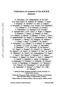
yield cs 2 = 0.5 (cs = 0.7). We choose u = 0.8. With the help of (37) we find λ = 1.7 f m for the soliton width and 0.6 for its amplitude. Even though this work is essentially qualitative the chosen numbers are well appropriate to study a realistic situation of a perturbation traversing the QGP. In Fig. 1 we show the numerical solution of (32) with initial condition ρˆ1 (x, t = 0) and ρˆ1 (x, t) given by (36). We can observe the time evolution of the initial gaussian-like pulse as a well defined soliton, keeping its shape and form. This solution shows the behavior expected from the analytic solution. We see that using the correct input for the amplitude and width we obtain a pulse which propagates without distortion. This initial condition is a very special case of little practical interest. A real perturbation produced in the QGP will most likely have the “wrong” amplitude and “wrong” width. For arbitrary amplitudes the solution must be numerically calculated. In Fig. 2 we show again the numerical solution of (32) with the initial condition given by (36) multiplied by a factor 10. Now we observe that the initial pulse starts to develop secondary peaks, which are called “radiation” in the literature. Further time evolution will increase the strength of these peaks until the complete loss of localization. In Fig. 3 we show the numerical solution of (35) with the initial condition given by (36). We observe the gradual formation of a “wall” followed by the dispersion of the initial pulse. In Fig. 4 the amplitude of the initial pulse (36) is multiplied by a factor 10 and used as initial condition for (35). As expected the dispersion takes place much earlier than in Fig. 3.
VI.
SUMMARY
The main conclusion of this work is that it is indeed possible to have KdV solitons in QCD, provided that two conditions are satisified. The first condition is that the gluon field have a dynamical mass. In this case the equation of motion (12) can be solved in the weak inhomogeneity approximation yielding (18). The existence of a dynamical gluon mass has been intensely discussed in the literature during the last years and seems to be well established (for details see the references given in [8]). For a massless gluon field we can only have a breaking wave equation, as it was found in our previous work [7]. The second condition is the existence of second order derivative terms in the energy density and 9
0,7
t=0 fm
0,6
t=50 fm 0,5
^
t=80 fm
0,4
0,3
0,2
0,1
0,0 0
10
20
30
40
50
60
70
80
x (fm)
FIG. 1: Numerical solution of (32) with (36) as initial condition calculated at different times.
t=0 fm
10
t=1 fm t=5 fm
8 ^
t=10 fm
6 4 2 0
0
10
20
30
40
x (fm)
FIG. 2: The same as Fig. 1 with an initial amplitude ten times larger.
pressure. These terms appear naturally from the formalism, as we can see in (15). However it is necessary to keep these derivative terms. The use of uniform field approximations prevents us from finding KdV solitons. If we neglect the derivatives we arrive at the breaking wave equation (35). The practical difference between perturbations governed by the KdV and BW equations is that the former propagate much longer keeping its localization whereas the latter loose localization and may generate unstable “walls”. The numerical analysis of some cases confirms the anticipated qualitative expectation. The application of the formalism 10
1,2
t=0 fm t=5 fm
1,0
t=10 fm t=15 fm
0,8
t=20 fm
^ 0,6
0,4
0,2
0,0 0
10
20
30
40
x (fm)
FIG. 3: Numerical solution of (35) with (36) as initial condition.
12 10
t=0 fm t=0.5 fm
8
t=1 fm
^
t=2 fm
6 4 2 0
0
5
10
15
20
x (fm)
FIG. 4: The same as Fig. 3 with an initial amplitude ten times larger.
developed in this work to problems in the theory of compact stars is in progress.
11
Acknowledgments
This work was partially financed by the Brazilian funding agencies CAPES, CNPq and FAPESP.
[1] P. G. Drazin and R. S. Johnson, “Solitons: An Introduction”, Cambridge University Press, 1989. [2] G.N. Fowler, S. Raha, N. Stelte and R.M. Weiner, Phys. Lett. B 115, 286 (1982); S. Raha, K. Wehrberger and R.M. Weiner, Nucl. Phys. A 433, 427 (1984); E.F. Hefter, S. Raha and R.M. Weiner, Phys. Rev. C 32, 2201 (1985). [3] D.A. Foga¸ca and F.S. Navarra, Phys. Lett. B 639, 629 (2006). [4] D.A. Foga¸ca and F.S. Navarra, Phys. Lett. B 645, 408 (2007). [5] D.A. Foga¸ca and F.S. Navarra, Nucl. Phys. A 790, 619c (2007); Int. J. Mod. Phys. E 16, 3019 (2007). [6] D.A. Foga¸ca, L. G. Ferreira Filho and F.S. Navarra, Nucl. Phys. A 819, 150 (2009). [7] D.A. Foga¸ca, L.G. Ferreira Filho and F.S. Navarra, Phys. Rev. C 81, 055211 (2010). [8] D.A. Foga¸ca and F.S. Navarra, Phys. Lett. B 700, 236 (2011). [9] S. Weinberg,“Gravitation and Cosmology”, New York: Wiley, 1972. [10] L. Landau and E. Lifchitz, “Fluid Mechanics”, Pergamon Press, Oxford, (1987). [11] L. S. Celenza and C. M. Shakin, Phys. Rev. D 34, 1591 (1986). [12] X. Li and C. M. Shakin, Phys. Rev. D 71, 074007 (2005). [13] B.D. Serot and J.D. Walecka, Advances in Nuclear Physics 16, 1 (1986). [14] R. C. Davidson, “Methods in Nonlinear Plasma Theory”, Academic Press, New York an London, 1972, pages 20 and 21.
12


![arxiv: v1 [physics.plasm-ph] 29 Jun 2015](https://kipdf.com/img/300x300/arxiv-v1-physicsplasm-ph-29-jun-2015_5aaf9acc1723dd329c6336ad.jpg)
![arxiv: v1 [cs.cv] 29 Jun 2016](https://kipdf.com/img/300x300/arxiv-v1-cscv-29-jun-2016_5ac1c4a51723ddaecd8b31cf.jpg)
![arxiv: v1 [astro-ph.co] 29 Jun 2012](https://kipdf.com/img/300x300/arxiv-v1-astro-phco-29-jun-2012_5aeda9397f8b9a72478b4600.jpg)
![arxiv: v1 [cs.cv] 29 Jun 2014](https://kipdf.com/img/300x300/arxiv-v1-cscv-29-jun-2014_5addd3367f8b9a55678b45a5.jpg)
![arxiv: v1 [nucl-th] 16 Jun 2011](https://kipdf.com/img/300x300/arxiv-v1-nucl-th-16-jun-2011_5ac4f7881723ddb7b6ca36ca.jpg)
![arxiv: v1 [cs.ds] 28 Jun 2011](https://kipdf.com/img/300x300/arxiv-v1-csds-28-jun-2011_5aad31231723dd8518aa3c37.jpg)
![arxiv: v1 [astro-ph.ga] 15 Jun 2011](https://kipdf.com/img/300x300/arxiv-v1-astro-phga-15-jun-2011_5b0da6358ead0e048d8b45eb.jpg)
![arxiv: v1 [astro-ph.co] 2 Jun 2011](https://kipdf.com/img/300x300/arxiv-v1-astro-phco-2-jun-2011_5ad810c37f8b9a748a8b45cf.jpg)
![arxiv: v1 [physics.flu-dyn] 9 Jun 2011](https://kipdf.com/img/300x300/arxiv-v1-physicsflu-dyn-9-jun-2011_5ad4b2df7f8b9a757f8b458b.jpg)
![arxiv: v1 [physics.class-ph] 11 Jun 2011](https://kipdf.com/img/300x300/arxiv-v1-physicsclass-ph-11-jun-2011_5ac2c2ca1723ddd37f687cce.jpg)
![arxiv: v1 [cs.dc] 29 Nov 2011](https://kipdf.com/img/300x300/arxiv-v1-csdc-29-nov-2011_5ac3c4391723dd706a2f1ced.jpg)
![arxiv: v1 [cond-mat.mes-hall] 28 Jun 2011](https://kipdf.com/img/300x300/arxiv-v1-cond-matmes-hall-28-jun-2011_5aaf77d41723dd339c802a7a.jpg)
![v1 [cs.ni] 29 Jun 2006](https://kipdf.com/img/300x300/v1-csni-29-jun-2006_5ac9b2291723dd99a7e69b61.jpg)
![arxiv: v1 [math-ph] 8 Jun 2007](https://kipdf.com/img/300x300/arxiv-v1-math-ph-8-jun-2007_5ab2d27b1723dd349c81287c.jpg)
![arxiv: v1 [cond-mat.soft] 22 Jun 2015](https://kipdf.com/img/300x300/arxiv-v1-cond-matsoft-22-jun-2015_5aabd0fd1723ddfa9258bb7b.jpg)
![arxiv: v1 [q-bio.nc] 18 Jun 2009](https://kipdf.com/img/300x300/arxiv-v1-q-bionc-18-jun-2009_5ab4fbea1723dd349c817eb3.jpg)
![arxiv: v1 [cs.cl] 22 Jun 2015](https://kipdf.com/img/300x300/arxiv-v1-cscl-22-jun-2015_5aacf8701723dd76651566d5.jpg)
![arxiv: v1 [astro-ph.sr] 30 Jun 2016](https://kipdf.com/img/300x300/arxiv-v1-astro-phsr-30-jun-2016_5aadcdf91723ddaf88aa1799.jpg)
![arxiv: v1 [math.co] 1 Jun 2013](https://kipdf.com/img/300x300/arxiv-v1-mathco-1-jun-2013_5aae00761723dd7a2c9b1c91.jpg)
![arxiv: v1 [gr-qc] 2 Jun 2012](https://kipdf.com/img/300x300/arxiv-v1-gr-qc-2-jun-2012_5ad54d237f8b9a934e8b4591.jpg)
![arxiv: v1 [astro-ph.co] 1 Jun 2010](https://kipdf.com/img/300x300/arxiv-v1-astro-phco-1-jun-2010_5ad9547d7f8b9a4a7b8b45cd.jpg)
![arxiv: v1 [cs.ne] 14 Jun 2016](https://kipdf.com/img/300x300/arxiv-v1-csne-14-jun-2016_5ad6ee5c7f8b9a840f8b461b.jpg)
![arxiv: v1 [astro-ph.sr] 15 Jun 2009](https://kipdf.com/img/300x300/arxiv-v1-astro-phsr-15-jun-2009_5ad423e67f8b9a6f0b8b4578.jpg)