CAS/CNS TR-2002-011
Parsons & Carpenter
1
ARTMAP neural networks for information fusion and data mining: Map production and target recognition methodologies Olga Parsons and Gail A. Carpenter Department of Cognitive and Neural Systems Boston University Boston, Massachusetts 02215
[email protected],
[email protected]
Neural Networks, in press Submitted: September, 2002 Revised: December, 2002
Technical Report CAS/CNS TR-2002-011 Boston, MA: Boston University
Running title: Map production methodologies Acknowledgements: This research was supported by grants from the Air Force Office of Scientific Research (AFOSR F49620-01-1-0397 and AFOSR F49620-01-1-0423) and the Office of Naval Research (ONR N00014-01-1-0624). Address correspondence to: Professor Gail A. Carpenter, Department of Cognitive and Neural Systems, 677 Beacon Street, Boston University, Boston, MA 02215.
[email protected]
CAS/CNS TR-2002-011
Parsons & Carpenter
2
ARTMAP neural networks for information fusion and data mining: Map production and target recognition methodologies
Abstract The Sensor Exploitation Group of MIT Lincoln Laboratory incorporated an early version of the ARTMAP neural network as the recognition engine of a hierarchical system for fusion and data mining of registered geospatial images. The Lincoln Lab system has been successfully fielded, but is limited to target / non-target identifications and does not produce whole maps. Procedures defined here extend these capabilities by means of a mapping method that learns to identify and distribute arbitrarily many target classes. This new spatial data mining system is designed particularly to cope with the highly skewed class distributions of typical mapping problems. Specification of canonical algorithms and a benchmark testbed has enabled the evaluation of candidate recognition networks as well as pre- and post-processing and feature selection options. The resulting mapping methodology sets a standard for a variety of spatial data mining tasks. In particular, training pixels are drawn from a region that is spatially distinct from the mapped region, which could feature an output class mix that is substantially different from that of the training set. The system recognition component, default ARTMAP, with its fully specified set of canonical parameter values, has become the a priori system of choice among this family of neural networks for a wide variety of applications. Keywords: ARTMAP; Adaptive Resonance Theory (ART); Information fusion; Data mining; Remote sensing; Mapping; Image analysis; Pattern recognition
1. Introduction Neural network models for vision, learning, and recognition form the foundation of a system for multisensor image fusion and data mining developed by Allen Waxman and colleagues, first in the Sensor Exploitation Group at MIT Lincoln Laboratory (Ross et al., 2000; Streilein et al., 2000; Waxman et al., 2001) and recently in the Boston University CNS Technology Lab (Waxman et al., 2002). While the primary domain of the Lincoln Lab (LL) system is geospatial image analysis, it has also been tested for other spatially defined applications, including medical imaging (Aguilar & Garrett, 2001). Fuzzy ARTMAP was chosen to perform category recognition and output class prediction in the LL fusion system because of its computational capabilities for incremental training, fast stable learning, and visualization. ARTMAP networks learn to predict specified output classes from critical patterns of input features, with the system creating as many of these internally defined categories as needed to meet accuracy criteria. The interpretability of the learned category structure with respect to input features suggests straightforward feature selection methods, which are often important for efficient on-line image processing and search of large images. Despite extensive development of other functions, the LL system still relies on the originally implemented simplified ARTMAP algorithm (Kasuba, 1993). Meanwhile, new ARTMAP systems that have been developed over the past decade include ART-EMAP (Carpenter & Ross, 1995), ARTMAP-IC (Carpenter & Markuzon, 1998), and distributed ARTMAP (Carpenter,
CAS/CNS TR-2002-011
Parsons & Carpenter
3
Milenova, & Noeske, 1998). Network capabilities and design options have been tested, and system performance has been compared with that of other neural and statistical algorithms, on many application domains, including remote sensing, data mining, and visualization (e.g., Carpenter et al., 1997, 1999; Gopal, Liu, & Woodcock, 2000; Gopal, Woodcock, & Strahler, 1999). The studies described in this paper have examined the performance of several ARTMAP networks in the context of the LL image mining system. To test candidate general-purpose algorithms, a challenge problem was constructed that specifies eight target classes and identifies a corresponding ground truth data set for an image on which the LL system had previously been demonstrated (Streilein et al., 2000). A systematic mapping methodology, alternative labeling protocols, post-classification adjustment techniques, and feature selection were also defined and tested. This standardized procedure assumes that training pixels come from an area that is spatially separate from the test region to be mapped, and that the training and testing regions typically contain different output class distributions. These methods extend the capabilities of the LL system, which is designed for one-class (target / non-target) labeling, to allow on-line learning of an arbitrary number of target classes and to produce whole maps. This investigation has identified a system, called default ARTMAP, that has produced accurate results on difficult recognition tasks while featuring comparative simplicity of design and robust performance in many application domains. An important aspect of this algorithm is its continuous-valued distributed predictions across target classes. Labels are chosen based on the sum of these distributions across a set of network voters, which learn with different orderings of a shared training set. ARTMAP variants with winner-take-all coding and discrete target class predictions, including the one implemented in the LL system, showed consistent deficits in labeling accuracy and post-classification map adjustment capabilities. The default ARTMAP algorithm and parameter values specified here define a ready-to-use general-purpose system for supervised learning and recognition. The paper is organized as follows. Section!2 introduces a prototype map containing three target classes, defines a protocol for systematic assessment of map creation methods, and defines the default ARTMAP algorithm. Section!3 illustrates alternative mapping methods on the prototype example. Section!4 describes the Monterey benchmark image to be used for evaluation of mapping methods, and demonstrates default ARTMAP performance and post-classification adjustment capabilities on this example. Section!5 evaluates the performance of a nested family of ARTMAP networks on the Monterey benchmark problem, Section!6 shows an eight-class map produced from the image, and Section 7 describes how feature selection can reduce the number of input components without loss of accuracy. Sections 8-11 specify algorithms for map production and classifier evaluation methodologies, default ARTMAP training and testing, and input feature selection.
2. Map production methodology A 1.5 million pixel image of the Monterey Naval Postgraduate School (Figure!1a) provided inputs to the benchmark testbed for classifier comparisons. In order to maintain a valid comparison of candidate recognition networks within the context of the LL spatial data mining system, this analysis uses the same feature vectors (produced by Mario Aguilar) as were used in previously published demonstrations of the Monterey image (Ross et al., 2000; Streilein et al., 2000; Waxman et al., 2001,2002). Specifically, the LL system describes each pixel as a 20dimensional feature vector: contrast-enhanced values (G,R,NIR,B) of the four original color
CAS/CNS TR-2002-011
Parsons & Carpenter
4
bands (green, red, near infrared, blue); eight single-opponent (G/R, R/G, NIR/B, B/NIR, G/NIR, G/B, R/NIR, R/B) and four double-opponent (G/R, R/G, NIR/B, B/NIR) measures of local color contrasts; three selected linear combinations of the four contrast-enhanced bands (G+R, NIR+B, G+R+NIR+B); and one height measure, obtained from low-level Digital Terrain Elevation Data. The contrast-enhanced color bands were computed by shunting center-surround processing (Grossberg, 1973) within each color layer. Measures of single- and double-opponent processing in the visual system (Lennie, 2000) were also modeled by center-surround networks, with contrast enhancement between bands (e.g., R center, G surround). In the LL system, surrounds are represented by a 7x7 matrix of pixels, and centers by the pixel at the center of this matrix. Figure!1 (a) Monterey image (b) Prototype image To construct a benchmark problem on which to test performance of supervised learning systems, eight target output classes (red cars, non-red cars, roofs, roads, foot paths, grass, trees, other) were specified, and ground truth pixel sets located, by observation of the Monterey image (Section 4). In order first to illustrate map production methodologies, a simplified testbed, called the prototype image (Figure!1b), with three target classes and 160,000 pixels, is first defined (Section!2.1). Section!2.2 outlines a cross-validation protocol for training, validation, and testing; and Section!2.3 characterizes the default ARTMAP system, which is used for classification on this example. Default ARTMAP will later be compared with other ARTMAP variations on the Monterey mapping task (Section 5). Section 2.4 describes how continuous-valued outputs are summed across voting networks to produce class predictions.
2.1. Defining the prototype map The prototype map was constructed using three of the Monterey class labels: trees, roads, and cars (non-red). Each pixel was assigned a 20-component feature vector corresponding to a pixel from the same class in the Monterey image. A majority of feature vectors assigned to contiguous pixels from a given class were drawn from contiguous pixels in the original image, although this approximate topography could not be fully preserved throughout the prototype map, especially for small objects (cars). Note that the prototype testbed retains a challenging feature found in many mapping problems, namely, an unbalanced distribution of target classes, with fewer than 1% of the pixels labeled car (Table!1). Table!1 Prototype image pixel distribution
2.2. Map production and classifier evaluation protocols A cross-validation procedure was defined for systematic assessment of map creation methods, candidate classifiers, post-processing techniques, and input feature selection. Each image was divided into four vertical strips. Training set pixels were drawn from two strips; a third strip provided a validation set for methods that required parameter selection; and pixels from the remaining strip were used for testing. As is typical for cross validation, training, validation, and testing sets are disjoint. In addition, the mapping protocol imposes a stricter standard, with pixels from the three sets drawn from spatially distinct regions. The procedure thus emulates the task of map production by a system trained and tested in geographically separate locations. Figure!2 Prototype image cross-validation strips
CAS/CNS TR-2002-011
Parsons & Carpenter
5
Vertical strips in the prototype map measure 100 ¥ 400 pixels (Figure!2). Table!1 shows the pixel distribution in each strip across the three target classes. One hundred pixels from each class were selected at random from each strip. This fixed set of designated pixels (0.75% of each strip) produced the training, validation, and testing sets for all prototype simulations.
2.3. The default ARTMAP classifier The classifier used for the prototype example is a version of the ART-EMAP network (Carpenter & Ross, 1995). This system, specified as an algorithm in Sections 9 and 10, codes the current input as a winner-take-all activation pattern during training and as a distributed activation pattern during testing. For distributed coding, the transformation of the filtered bottom-up input to an activation pattern across a field of nodes is defined by the increased-gradient CAM rule (Carpenter, Milenova, & Noeske, 1998). The network also implements the MT– search algorithm (Carpenter & Markuzon, 1998), with the baseline vigilance parameter set equal to zero, for maximal code compression. Other ARTMAP design choices for default ARTMAP include fast learning, whereby weights converge to asymptote on each learning trial; single-epoch training, which emulates on-line learning; and a choice-by-difference signal function (Carpenter & Gjaja, 1994) from the input field to the coding field. When a supervised learning problem has more than two output classes, a single system may be trained to predict all the classes at once. Alternatively, multiple systems, one for each output class, can each be trained to make a target / non-target decision. In the latter case, test set predictions pool output activations of all trained networks. Results for the prototype map reported here are obtained from a single network trained on three output classes. For the Monterey benchmark problem, results of training on both eight-class networks and groups of eight target / non-target networks are compared. When, as is generally the case for the mapping problems considered here, the two training strategies produce similar results, the single-network strategy has the advantage of simplicity.
2.4. Distributed voting ARTMAP’s capacity for fast learning implies that the system can incorporate information from examples that are important but infrequent and can be trained incrementally. Fast learning also causes each network’s memory to vary with the order of input presentation during training. Voting across several networks trained with different orderings of a given input set takes advantage of this feature, typically improving performance and reducing variability as well as providing a measure of confidence in each prediction (Carpenter et al., 1992). While the number of voting systems is, in general, a free parameter, five voters have proven to be sufficient for many applications. This a priori choice of five voting systems (for each training set combination) was used in all studies described here. Even with the number of voters fixed, other design choices appear in systems where output activations may be distributed. In particular, default ARTMAP, which produces a continuousvalued distribution s k across target classes k for each test set item, presents options for combining weighted predictions across voters to make a final class choice. One strategy sums the s k values of individual networks to produce a net distributed output pattern, which is then used to determine the predicted class. An alternative strategy first lets each voting network choose its own winning output class, then assigns the test set inputs on the basis of these individual votes.
CAS/CNS TR-2002-011
Parsons & Carpenter
6
In most applications, the first of these two voting strategies produces better results. This was also found to be the case in pilot studies for the current mapping problem, with the second strategy showing poorer performance on under-represented classes. Thus in all simulations reported here target class decisions are based on the distributed output sum of all voting networks. In fact, the continuous nature of distributed output class predictions will prove to be an essential characteristic of the default ARTMAP system.
3. Assigning target class labels Assume now that voting networks have been trained on different orderings of a given set of labeled pixels drawn from two vertical strips in an image, and that the output patterns s k have been summed across voters for each pixel to be labeled. This section!examines methods for using the summed output activation patterns to produce a map by assigning class labels to each pixel in the image.
3.1. Three methods for choosing target class labels A natural method for producing a class label for an input pixel takes the predicted class to be the one with the largest summed output. However, this method may produce target class representations in the resulting map that are far from their true proportions. A second class label selection method imposes a prior class distribution estimate, when this information is available. A third method uses a validation procedure to bias labeling decisions. Note that, for each test set input, all three methods operate on the same output class distribution pattern, which is equal to the summed predictions of the previously trained voting networks. We now consider the performance of these three class label assignment procedures on the prototype mapping problem. For each, the training set consists of 200 pixels per class, from two strips. Reported results (hit and false alarm rates) are averages across the six possible combinations of two strips that provide training set pixels for each simulation. In addition to using quantitative measures such as test-set accuracy, maps can be evaluated qualitatively, in terms of appearance and utility. For this purpose, images of whole labeled prototype maps are produced by training on the designated pixels subsets from strips!1, 2, and 4.
3.1.1. Baseline method The baseline method labels each pixel as belonging to the output class k with the largest sum of predictions s k . This method uses neither prior class distribution estimates nor parameter selection by validation. Table 2a shows hit and false alarm rates produced by the baseline method on test set strips of the prototype image, averaged across the six training strip † combinations. These results indicate that the straightforward baseline method for target class labeling produces reasonable hit and false alarm rates on test set pixels. The statistics are misleading, however, as is often the case for classification problems with highly skewed class label distributions. In fact, the baseline method labels 4.9% of test strip pixels as cars, which is more than six times the fraction of actual car pixels (0.75%) in the true image (Table!1). Overproduction of labeled car pixels is clearly visible in the baseline map (Figure 3a, upper row), even without knowledge of their true proportion. Table!2 Prototype map classes from (a) baseline, (b) prior probabilities, and (c) validation methods
CAS/CNS TR-2002-011
Parsons & Carpenter
7
Figure!3 Prototype map class labels A confusion matrix (Table 3) for one typical combination (training on strips 1 and 4, testing on strip 3) provides additional details about the pattern of class labeling errors. Rows in Table 3a show the output class predictions for the 100 test set pixels that actually belong to each class. Diagonal terms, equal to the numbers of correctly labeled pixels, show that the class-specific (98 / 84 / 95%) and overall (92.3%) accuracy rates on this strip are close to the corresponding average rates (98.3 / 84.0 / 95.0% and 92.4%) in the first row of Table 2a. Similarly, off-diagonal terms in the confusion matrix generate false alarm rates. For example, the third column shows that 18 of the 200 non-car pixels in the test strip are incorrectly labeled car, producing a false alarm rate of 9% for this class. The false alarm rates for this combination (1 / 1.5 / 9%) are again close to the corresponding average rates (1.3 / 1.3 / 8.8%) from the six training strip combinations. Table!3 Baseline method confusion matrix Although entries in the 3¥ 3 confusion matrix show cross-class error patterns only on the 300 test set pixels in strip 3, this information can be combined with knowledge of actual class distributions to estimate the fractions of each output class that this trained system would produce on all 40,000 pixels in the strip. Namely, multiplying the row vector of a priori class distributions (78.47 / 21.11 / 0.42%) for strip 3 (Table 1) by the confusion matrix produces an estimate of this strip’s predicted whole-map class distribution pattern (76.4 / 17.7 / 5.9%), which is close to the average class distribution pattern (77.6 / 17.6 / 4.9%) predicted by the baseline method, as shown in the last row of Table 2a.
3.1.2. Prior probabilities method Where a known or estimated distribution of target classes in the whole map is available, a prior probabilities method may be used to bias class label assignments to match the specified output class distribution. At each step in this map labeling process, a target class is selected at random according to the a priori distribution. The still-unlabeled pixel with maximum activation for the selected class is assigned that class label. Compared to the baseline method, labeling with prior probabilities misses more true car pixels in the prototype map, reducing the hit rate to 75.0% (Table!2b). However, the represented proportion (0.76%) of the class cars is now correct. The improved appearance of the whole map, visible in Figure!3b, must be attributed in part to the fact that this method supplies more information to the classifier, in the form of the true class distribution. Even when it is not possible to estimate in advance an approximate target class distribution, a user can still make use of the prior probabilities method to improve the appearance of a labeled map. Suppose, for example, that a map produced by the baseline method appears, upon visual inspection, to have too many car pixels. The user can then adjust the pixel distribution initially produced by that method (as in Table!2a) to specify a new distribution for the prior probabilities method, and can continue to balance a priori target classes until the appearance of the map becomes satisfactory. A graphics tool that overlays the labeled map on the original image one class at a time assists the estimation process, especially for sparsely represented classes. Since all labeling methods begin with the same summed output patterns from the already trained networks, iterations of the final labeling methods are rapid and straightforward.
CAS/CNS TR-2002-011
Parsons & Carpenter
8
3.1.3. Validation method The validation method adjusts class label percentages without requiring a priori estimation of their true distribution in the map. Rather, this method allows the user to bias the labeling process by checking outcome statistics on a validation set. The method used here introduces output class decision thresholds as new free parameters, and estimates their values from the validation strip, which was not used by the baseline and prior probabilities methods. An alternative method could adapt ARTMAP output class weights W jk by gradient descent, as in Carpenter, Milenova, and Noeske (1998). All three methods begin with the same output distribution across target classes computed by the trained voting system. For a given pixel, let s f denote the fraction of this distribution assigned to the class label f . Whereas the baseline and prior probabilities methods assign class labels according to values of s f , the validation method assigns the label so as to maximize the amount by which s f exceeds a class-specific decision threshold g f . Decision thresholds are computed one class at a time, as follows. The baseline method assigns a pixel to a target class f whenever s f is maximal. This corresponds to the validation method with all decision thresholds set equal to zero. Imagine, now, biasing the system against choosing one particular class f by replacing s f with s f - g .
(
Increasing g reduces the fraction of validation set pixels HitRateg
(
)
(
)
) correctly predicting class
f , but it also reduces the fraction of pixels FalseAlarmg predicting f that actually belong to a different class. As g increases parametrically from 0 to 1, the graph of HitRateg as a function of FalseAlarmg traces an ROC curve. The decision threshold g = g f is chosen so as to
(
)
maximize the difference HitRateg - FalseAlarmg on the validation set. This choice corresponds to the point where the ROC curve intersects the highest possible line with unit slope. Once a decision threshold has been set for each class, pixels are labeled as the target class f that maximizes sf - gf .
(
)
Additionally, this method specifies an upper bound on the estimated false alarm rate for each class: if the chosen threshold produces a false alarm rate higher than 10% on the validation set, its†value is raised until the false alarm rate falls to just below 10%. An upper bound helps ensure that classes with few pixels in the true map are not over-represented in the labeled map. For example, on six training set combinations of one typical prototype simulation, the validation method produced decision thresholds g cars between 0.085 and 0.165, while g trees and g roads each remained equal to 0 for all but one combination. As shown for the Monterey map below, designated upper bounds can also be adjusted for certain target classes, to balance their representation in the whole map. As with prior probabilities, iterative corrections by visual inspection of maps produced by the validation method are rapid and easy to test. Table!2c shows that validation produces the best overall predictive accuracy (94.4%) of all the methods. Despite being given no prior information about class probabilities, this method † produced a class distribution that was much improved compared to the baseline method. Nonetheless, the validation method labeled as cars over twice as many test pixels as in the true † † †
CAS/CNS TR-2002-011
Parsons & Carpenter
9
map, a trend that can also be seen by comparing the labeled whole maps in the upper row of Figures 3b and 3c.
3.2. Post-processing a labeled map The methods described in Section!3.1, which label pixels independently, tend to produce speckle in the final maps (Figure!3, upper row). Post-processing can improve both test-set classification performance and the look of a map. Standard post-processing techniques include averaging, smoothing filters, and morphological operations (e.g., Shapiro & Stockman, 2001; Matlab Image Processing Toolbox, http://www.mathworks.com/access/helpdesk/help/toolbox/ images/images.shtml). Post-processing by a simple voting filter is tested here. Namely, each pixel assumes the label originally assigned to the majority of abutting pixels (eight neighbors) plus three copies of itself, with ties broken in favor of the class with the fewest pixels in the original labeling. Table!4 Prototype map classification with post-processing Comparing Table!4 with Table!2 shows that post-processing the prototype map by the averaging filter increased the overall pixel-by-pixel test-set accuracies for all three methods. Postprocessing also brought the fraction that the baseline and validation methods assigned to the difficult under-represented class cars closer to that of true map (0.75%). A comparison of the upper and lower rows of Figure!3c illustrates how post-processing can reduce speckle in maps produced by the validation method. Post-processing tends to be even more effective on real images than on the prototype. This is due to a construction artifact of the prototype image, where a substantial fraction of feature vectors for neighboring pixels in small objects (cars) were drawn from spatially separated objects in the source Monterey image, thereby reducing the meaning of spatial contiguity in this example. In addition, whereas the a priori class distribution is exact in the prototype example, errors in the distribution estimates for real images produce additional mapping errors which can be usefully corrected at a post-processing stage.
4. The Monterey benchmark mapping problem The methods illustrated on the prototype example will now be used to compare candidate ARTMAP classifier modules and to produce a labeled map of the Monterey location. To prepare for training, validation, and testing, a ground truth dataset was created by visual inspection of the original image (Figure!1a). Pixels or regions were assigned labels from eight target classes: red cars, non-red cars, roofs, roads, foot paths, grass, trees, other. The total number of pixels labeled was 225,828, covering about 15% of the image. In synthetic examples such as the prototype map (Section 2), the true distribution of classes is known by construction. In most real examples, where ground truth typically covers only a small fraction of the image, global class distributions are not known. In order still to be able to test a priori distribution methods (Section!3.1.2), approximate class distributions were obtained by visual inspection of the Monterey image. Because such estimates are typically imprecise, distributions calculated independently by eight observers were averaged (Table!5). Table!5 Monterey class distribution estimates To prepare for cross validation, the Monterey image was partitioned into four vertical strips. If available, 250 pixels were randomly selected and fixed for each class in each strip. If a strip
CAS/CNS TR-2002-011
Parsons & Carpenter
10
contained fewer labeled pixels for a particular class, then all available pixels were chosen. On average, 1,738 pixels of the 372,592 in each strip constituted the training / validation / test set.
4.1. Default ARTMAP performance on the Monterey example Table 6a-c summarizes the results of applying the mapping methodologies developed in Sections 2 and 3 to the Monterey image, using default ARTMAP without post-processing. Comparing the class distribution statistics in Table 6 with Table 5 shows that, as on the prototype map (Table 2), the baseline and validation methods label too many pixels as belonging to under-represented classes (e.g., red cars, non-red cars, foot paths), generally at the expense of roofs and roads. Validation has the greatest effect on non-red cars, where positive decision thresholds in five of the six training combinations eliminated about half of the over-representation of that class, transferring most to the adjacent road pixels. Table!6 Monterey map classification
4.2. Post-classification adjustments Post-processing by a voting filter (Section 3.2) improves the overall accuracy of all three methods by about 2%, but has a negligible effect on class distributions. A more important benefit of post-processing is removing speckle from the labeled image. This is particularly true for the prior probabilities method (Figure 4a), where the approximate nature of initial distribution estimates leads to forced over-labeling of over-estimated classes. Figure!4 Class adjustment via (a) post-processing, (b) class %, (c) false alarm rate In addition to locally defined post-processing, the prior probability and validation methods allow the user to make rapid adjustments to balance map classes. After a map has been generated, the user can view the results of classification and decide whether adjustments are needed. Figure 4 shows the result of adjusting a class percentage with the prior probabilities method (Figure 4b) and of adjusting an upper bound on the false alarm rate with the validation method (Figure 4c). An effective way to visualize per class performance is to overlay the results of recognition on the original image one class at a time. The left image of Figure 4b shows the classification results for roofs in a portion of the Monterey image. Here, a majority of roof pixels are labeled correctly but some tree and road pixels are also labeled as roof. After the roof percentage was reduced from 30% to 14%, most incorrectly labeled pixels disappeared, as seen in the right image of Figure 4b. Post-classification visualization helps the user to correct errors in initial estimates of class distributions, which can vary widely (Table 5). Similar adjustments can be performed with the validation method. At the beginning, maximum false alarm rates were set to 10% for all classes. The result of the label assignment for non-red cars with this constraint is illustrated in the left image of Figure 4c. In the whole map, more than twice as many pixels as desired were labeled as non-red cars. The map was corrected by lowering the upper bound on the false alarm rate for non-red cars. When the false alarm rate was lowered from 10% to 0.2%, the map became more accurate as shown in the right image of Figure 4c. Table 6d also shows that adjusting maximum false alarm rates with the validation method can bring class distributions closer to their target values.
CAS/CNS TR-2002-011
Parsons & Carpenter
11
5. Evaluating ARTMAP classifiers and map production methods on the Monterey benchmark The studies described in this section compare performance of ARTMAP variants on the Monterey benchmark problem. The learning systems under consideration differ primarily in terms of their code representations (distributed vs. winner-take-all) during training and testing. Tested systems include a straightforward fuzzy ARTMAP network and the variant used in the Lincoln Lab implementation (LL), both of which employ winner-take-all coding during training and testing; default ARTMAP, which is the same as fuzzy ARTMAP during training but uses a distributed code representation during testing; ARTMAP-IC, which equals default ARTMAP plus instance counting, which biases a category node’s test-set output by the number of trainingset inputs coded by that node; and distributed ARTMAP, which employs a distributed code (and instance counting) during both training and testing. The versions of these networks tested here form a nested sequence: fuzzy ARTMAP Ã default ARTMAP Ã ARTMAP-IC Ã distributed ARTMAP That is, distributed ARTMAP reduces to ARTMAP-IC when coding is set to winner-take-all during training; ARTMAP-IC reduces to default ARTMAP when counting weights are set equal to 1; and default ARTMAP reduces to fuzzy ARTMAP when coding is set to winner-take-all during testing as well as training. The LL system incorporates the original fuzzy ARTMAP algorithm (Carpenter et al., 1992) as codified in a simplified form by Kasuba (1993). This algorithm differs somewhat from the version of fuzzy ARTMAP described above in that it uses the MT+ search algorithm (instead of MT–), a Weber Law choice function (instead of choice-by-difference), and exhaustive search of learned categories before activating an uncommitted node. Additional variations in the LL system include the use of two training epochs; two baseline vigilance values, a higher one for targets and a lower one for non-targets; and a discrete-valued confidence measure that is finer than a simple count of winner-take-all voters. Despite these additions, performance of the LL system on the Monterey map benchmark was found to be similar to that of the basic fuzzy ARTMAP network. In order to identify eight map classes, the LL system needs to train eight individual networks on target / non-target recognitions. All other networks are tested both with this method and with single-system training for eight outputs classes. Table 7 shows class distribution predictions made by the networks under consideration, each using the baseline method for class labeling without post-processing. Boldface entries indicate which predictions are closest (over- and/or under-estimates) to the average a priori class distribution of the Monterey image (Table 5). Although the distribution pattern produced by ARTMAP-IC is closest to the target, all the networks produce class label percentages that differ from the estimates. Therefore the prior probabilities method was selected for making a valid choice among classifiers. This labeling method evaluates test-set hit rates with class distribution patterns held constant. Table!7 Class distribution predictions of ARTMAP variations with the baseline method
CAS/CNS TR-2002-011
Parsons & Carpenter
12
Table 8 shows that the continuous-valued classifiers consistently produced the highest classspecific and overall accuracies. For the discrete-valued LL and fuzzy ARTMAP networks, ties frequently needed to be broken among classes with equal output values, which also produced speckle in the corresponding maps. Although the LL system adds intermediate confidence values to the voting system, which would seem to produce outputs more like those of the continuousvalued systems, this addition did not improve performance over that of basic fuzzy ARTMAP with five binary-valued voters. Output ties also created speckle in maps produced by fuzzy ARTMAP or the LL system. Table!8 Predictive accuracy of ARTMAP variations with the prior probabilities method Default ARTMAP and ARTMAP-IC (both 1- and 8-system versions) produced overall average test-set accuracies several points above those of the discrete-valued systems. Performance of 1system distributed ARTMAP was also close to that of default ARTMAP, but performance dropped markedly for the 8-system version, where coding can be unpredictable on the target / non-target discrimination tasks and where performance also varied dramatically from one strip to the next. Continuous-valued networks have the added benefit of superior class adjustment capabilities (Figure 4b,c). The instance counting feature of ARTMAP-IC adds a processing complexity to the default ARTMAP network, as does training a target / non-target network for every output class. In addition, instance counting may introduce sensitivity to numbers of training samples presented for each class. Thus, given their similar test-set accuracies, onesystem default ARTMAP was chosen as the network standard. The mapping problem considered here is sufficiently general as to recommend this system as the starting point for applications.
6. Producing a whole map Figure 5 shows a whole map of the eight Monterey classes produced by the validation method, after training one default ARTMAP system to label eight target classes. Training pixels were drawn from strips!1, 2, and 4, and validation pixels from strip!3. While training and validation pixels are included in the whole map, their sum constitutes only 0.35% of all pixels. The map was also post-processed with a voting filter. Figure!5 Monterey map, with default ARTMAP, validation method, post-processing With maps evaluated by visual inspection, one-system and eight-system default ARTMAP appeared to perform better than other candidates. Both prior probability and validation methods gave reasonable results without user adjustments, though the tuning of method parameters (a priori class distributions or maximum false alarm rates) improved the maps visibly. As in Figure 4a, maps produced by prior probabilities benefited most from post-processing by a voting filter, since they almost always contain speckle produced by errors in class distribution estimates. Maps produced by validation also improved with post-processing but this step was not essential. A map produced by the LL system contained a lot of speckle. Post-processing removed some of the speckle but sacrificed details. The problem of speckle can be traced to winner-take-all coding, which implies that the summed system output assumes at most twenty possible values.
7. Selecting input features In order to decrease the time required to identify target pixels in an entire image, the LL system is designed to select a subset of input features for the search, based on a criterion of maintaining performance on training pixels (Streilein et al., 2000). Feature selection also identifies which
CAS/CNS TR-2002-011
Parsons & Carpenter
13
data layers are important for defining objects of interest. The LL feature selection method uses an algorithm similar to one developed for ARTMAP systems in the context of medical database analysis (Carpenter & Milenova, 2000). These selection algorithms use the fact that, in a network trained with complement coded inputs, each feature of a learned category is represented as an interval of values. The algorithms calculate interval overlap of target vs. non-target nodes for each feature, delete features with the greatest interval overlaps, and retrain using subsets of the original feature set. The LL algorithm starts with the most promising feature, then adds others one by one while calculating training set performance. Only features that incrementally improve performance are retained. This section evaluates this method and extends it from the target / nontarget setting to systems with arbitrarily many output classes, with features selected on a validation set. Section 11 specifies this algorithm. The feature selection method tested with the default ARTMAP system identified 11 components of the Monterey input vector as the most useful across six training set combinations. Selected features were: 5 single-opponents (G/R, B/NIR, G/NIR, G/B, R/NIR), 3 double-opponents (G/R, R/G, NIR/B), 2 linear combinations (NIR+B, G+R+NIR+B), and height. It is interesting to note that the four individual contrast-enhanced color bands (G, R, NIR, B) were almost never chosen. Table 9 shows that the system trained and tested using only the 11 selected input components produced performance that was better than (or equal to) that of the same system using all 20 of the original features in all categories. Table 9 Feature selection Feature selection is one way in which the structure of ARTMAP memories supports interpretation and analysis. Further development of rule-based methods for spatial data mining is the subject of ongoing research.
8. Mapping methodology The following steps outline a procedure for labeling an arbitrary number of object classes in an image. Options include production of a whole map or evaluation of candidate classifiers on disjoint training and testing sets. Each image pixel is represented by a feature vector which may have an arbitrary number of feature components.
Map labeling and adjustment procedure 8.1. 8.2. 8.3. 8.4. 8.5. 8.6.
Define object classes for the image to be mapped. Estimate the a priori distribution of classes in the image. If not provided, create a ground truth set for each class by assigning labels to selected regions of the image. Divide the image into four strips, choosing vertical or horizontal to balance class distributions across strips. In each strip, randomly choose P labeled pixels for each class (or all pixels in a given class if fewer than P have been labeled). Fix five randomly chosen orderings of designated pixels in each strip. Choose training, validation, and testing strips: 8.6.a. For labeling a whole map: Choose three strips for training and one for validation. 8.6.b. For classifier evaluation: Choose two strips for training, one for validation, and one for testing.
CAS/CNS TR-2002-011 8.7. 8.8. 8.9. 8.10. 8.11.
8.12.
8.13.
Parsons & Carpenter
14
Train V systems (voters), each with E presentations of input vectors from one of the ordered pixel sets. For each voter, choose parameters by validation (if required). Present to each voter all pixels to be labeled in the whole map (mapping) or in the test strip (evaluation). Produce output class predictions s k for each pixel (Section 9). Sum the distributed output class predictions across the V voters. Label pixels by one of three methods (breaking ties by random choice): 8.11.a. Baseline: Assign the pixel to the output class k with the largest summed prediction. 8.11.b. Prior probabilities: Select an output class at random according to the estimated a priori distribution in the image. Assign that class label to the still-unlabeled pixel with the largest summed prediction for this class. 8.11.c. Validation: Bias the summed output class distribution, evaluating performance on the validation set. In this paper, decision thresholds are selected for each output class (Section 3.1.3), with an upper bound of 10% set for each false alarm rate. Alternatively, the distributed prediction of each voter (or of the sum) could be weighted by a steepest descent algorithm. Use the biased summed distribution to label the pixel by the baseline or prior probabilities method. Map adjustment: 8.12.a. Local image processing: Post-processing for speckle removal may be implemented as a simple voting filter, which assigns to each pixel the label originally assigned to a majority of its eight neighbors plus three copies of itself. 8.12.b. Class distribution adjustment: Starting with the output class predictions produced by any method (Step 8.11), target distribution percentages may be adjusted up or down (e.g., based on inspection of the resulting map), and class labels recomputed by the prior probabilities method. 8.12.c. False alarm rate adjustment: A decision threshold for an over-represented class may be increased to reduce the validation set false alarm rate. Classifier evaluation: Compute average performance statistics across six combinations of two training strips (each with five voters). Classifier evaluation measures include test strip output class distributions, hit and false alarm rates for each class and overall accuracy on the test set, performance variability between tasks, map appearance (overall and by overlays for each class), and degree of improvement by post-processing.
9. Default ARTMAP training The default ARTMAP algorithm specified here is a special case of the distributed ARTMAP (dARTMAP) algorithm described in Carpenter, Milenova, and Noeske (1998). Table 10 Default ARTMAP notation Table 11 Default ARTMAP parameter values
Default ARTMAP training (with winner-take-all code representation) 9.1.
Complement code M-D feature vectors a to produce 2M-D input vectors A: A ≡ a,ac and A = M
( )
9.2. 9.3.
Set initial values: wij = 1, W jk = 0 , C = 1 Select the first input vector A, with associated output class K
†
CAS/CNS TR-2002-011 9.4.
9.5. 9.6. 9.7.
Parsons & Carpenter
Set initial weights for the newly committed coding node j = C : wC = A WCK = 1 Set vigilance to its baseline value (r = r ) and set y = 0 Select the next input vector A, with associated output class K (until the last input of the last training epoch) Calculate signals to committed coding nodes j = 1KC:
(
9.8. 9.9.
15
)
T j = A Ÿ w j + (1- a ) M - w j Search order: Sort committed coding nodes with T j > aM in order of T j values (max to min) Search for a coding node that meets the matching criterion and makes the correct output class prediction: 9.9.a. Code: For the next sorted coding node ( j = J ) that meets the matching criterion Ê A Ÿ wJ ˆ ≥ r˜ , set y J = 1 (WTA) ÁË M ¯ C
9.9.b.
Output class predictions: s k =
 W jk y j = WJk j =1
9.9.c
9.10. 9.11.
Match tracking: If the active code fails to predict the correct output class Ê ˆ AŸw (s K = 0) , raise vigilance Á r = M J + e ˜ . Ë ¯ Return to Step 9.9.a (continue search). new old old Learning: Update coding weights: wJ = b A Ÿ wJ + (1- b )wJ .
(
)
Return to Step!9.5 (next input). After unsuccessfully searching the sorted list, increase C by 1. Return to Step 9.4 (add a committed node).
10. Default ARTMAP testing Default ARTMAP testing (with distributed code representation) 10.1. 10.2. 10.3. †10.4.
Complement code M-D feature vectors a to produce 2M-D input vectors A Select the next input vector A, with associated output class K Set y = 0 Calculate signals to committed coding nodes j = 1KC:
(
T j = A Ÿ w j + (1- a ) M - w j 10.5. 10.6.
)
{
}
Let L = {l = 1KC: Tl > aM } and L¢ = {l = 1KC: Tl = M} = l = 1KC: w j = A Increased Gradient (IG) CAM Rule: 1 10.6.a. Point box case: If L¢ ≠ f (i.e., w j = A for some j), set y j = for each L¢ j ŒL ¢
CAS/CNS TR-2002-011
Parsons & Carpenter
16
p
10.6.b.
È 1 ˘ Í ˙ ÍÎ M - Tj ˙˚ If L¢ = f , set y j = p for each j ŒL È 1 ˘ Â Í M - Tl ˙˚ l ŒL Î C
10.7.
Calculate distributed output class predictions: s k =
 W jk y j j =1
10.8. 10.9.
Until the last test input, return to Step!10.2 Predict output classes from s k values, according to chosen labeling method (see Step!8.11)
11. Feature selection Feature selection methods may be employed after an ARTMAP system has been trained on complete input vectors. The algorithm is based on methods, developed by Carpenter and Milenova (2000) and Streilein et al. (2000), which respect the geometry of ARTMAP memory representations.
11.1. D(k i ) : Diffentiability of class k by feature i D(k i ) indicates how well the feature i alone differentiates the output class k from all the
[
]
other classes. It is based on the degree of overlap of the weight intervals wiJ ,wic+ M ,J of
[
]
coding nodes J predicting k (W Jk = 1) with weight intervals wij ,wic+ M , j of coding
(
)
nodes j predicting all other classes W jk = 0 . Smaller overlaps (or disjoint intervals) correspond to higher degrees of differentiability. For each output class k and each feature i let: È wi + M ,J - wi + M , j + wiJ - wij D(k i ) = Â Í Í J :W Jk =1 Î 1- wi + M ,J Ÿ wi + M , j - wiJ Ÿ wij j:W jk =0
(
) (
)
˘ ˙ ˙ ˚
11.2. D(i) : Differential power of feature i For each class k, order the M input features i based on the values D(k i ) (max to min), and let O( k i ) equal the position of feature i in the ordered list for class k. 1 For each feature i, let the differential power D(i) = Â . O k i ( ) k Order features i based on their D(i) values.
11.3. U(i ) : Marginal predictive utility of feature i Derive an index set F of features i that show marginal predictive utility U(i ) on the validation set. Features are tested one at a time, in order of their differential power D(i) .
†
CAS/CNS TR-2002-011
Parsons & Carpenter
17
i , where i is the feature with largest D(i) . Test validation set performance with Let F = {} only component i presented in the input vector. Let U(i ) equal the number of validation samples classified correctly. Let i be the index with the next greatest D(i) . Test validation set performance with only components F » {} i presented in the input vector. Let U(i ) equal the number of validation samples classified correctly, less the number that were classified correctly with only input components F . Add i to F if U(i ) ≥ 1. Continue until U(i ) has been computed for all M input features.
11.4 Final selection of features Features are ordered and tested for each voter of each training set. Features are selected according to their high utility values and frequency of use. In Section 7, selected features were defined as those that had a marginal predictive utility U(i ) greater than half the maximum value for any training set; or were identified as useful (U (i ) ≥ 1) by all five voters on two or more training sets. These criteria can be adjusted by the user to increase or decrease the number of selected features.
References
†
†
†
Aguilar, M., & Garrett, A.L. (2001). Biologically-based sensor fusion for medical imagery. In Proceedings of SPIE Sensor Fusion: Architectures, Algorithms, and Applications Conference, Orlando, Florida. Carpenter, G.A., & Gjaja, M.N. (1994). Fuzzy ART choice functions. In Proceedings of the World Congress on Neural Networks (WCNN-94) (pp. 713-722), vol. I. Lawrence Erlbaum Associates. Carpenter, G.A., Gjaja, M.N., Gopal, S., & Woodcock, C.E. (1997). ART neural networks for remote sensing: Vegetation classification from Landsat TM and terrain data. IEEE Transactions on Geoscience and Remote Sensing, 35, 308-325. Carpenter, G.A., Gopal, S., Macomber, S., Martens, S., & Woodcock, C.E. (1999). A neural network method for mixture estimation for vegetation mapping. Remote Sensing of Environment, 70, 138-152. Carpenter, G.A., Grossberg, S., Markuzon, N., Reynolds, J.H., & Rosen, D.B. (1992). Fuzzy ARTMAP: A neural network architecture for incremental supervised learning of analog multidimensional maps. IEEE Transactions on Neural Networks, 3, 698-713. Carpenter, G.A., & Markuzon, N. (1998). ARTMAP-IC and medical diagnosis: Instance counting and inconsistent cases. Neural Networks, 11, 323-336. Carpenter, G.A., & Milenova, B.L. (2000). ART neural networks for medical data analysis and † fast distributed learning. In H. Malmgren, M. Borga, & L. Niklasson (Eds.), Artificial neural networks in medicine and biology (pp. 10-17). Springer series Perspectives in Neural Computing, London: Springer-Verlag. Carpenter, G.A., Milenova, B.L., & Noeske, B.W. (1998). Distributed ARTMAP: a neural network for fast distributed supervised learning. Neural Networks, 11, 793-813.
CAS/CNS TR-2002-011
Parsons & Carpenter
18
Carpenter, G.A., & Ross, W.D. (1995). ART-EMAP: A neural network architecture for object recognition by evidence accumulation. IEEE Transactions on Neural Networks, 6, 805-818. Gopal, S., Liu, W.G., & Woodcock, C. (2000). Visualization based on the Fuzzy ARTMAP neural network for mining remotely sensed data. In H.J. Miller & J. Han (Eds.), Discovering Geographic Knowledge in Data-rich Environments, Heidelberg: SpringerVerlag. Gopal, S., Woodcock, C., & Strahler, A. (1999). Fuzzy ARTMAP classification of global land cover from the 1 degree AVHRR data set. Remote Sensing of Environment, 67, 230-243. Grossberg, S. (1973). Contour enhancement, short-term memory, and constancies in reverberating neural networks. Studies in Applied Mathematics, 52, 217-257. Kasuba, T. (1993). Simplified Fuzzy ARTmap. AI Expert, 8(11), 18-25. Lennie, P. (2000). Color vision. In E.R. Kandel, J.H. Schwartz, & T.M. Jessell (Eds.), Principles of Neural Science, Fourth Edition (pp. 572-589). New York: McGraw-Hill. Ross, W.D., Waxman, A.M., Streilein, W.W., Aguilar, M., Verly, J., Liu, F. Braun, M.I., Harmon, P., & Rak, S. (2000). Multi-sensor 3D image fusion and interactive search. In Proceedings of 3rd International Conference on Information Fusion, Paris, vol. I. Shapiro, L., & Stockman, G. (2001). Computer Vision. New York: Prentice-Hall. Streilein, W., Waxman, A., Ross, W., Liu, F., Braun, M., Fay, D., Harmon, P., & Read, C.H. (2000). Fused multi-sensor image mining for feature foundation data. In Proceedings of 3rd International Conference on Information Fusion, Paris, vol. I. Waxman, A.M., Verly, J.G., Fay, D.A., Liu, F., Braun, M.I., Pugliese, B., Ross, W.D., & Streilein, W.W. (2001). A prototype system for 3D color fusion and mining of multisensor/ spectral imagery. In Proceedings of 4th International Conference on Information Fusion, Montreal, (pp. 3-10), vol. I. Waxman, A.M., Fay, D.A., Rhodes, B.J., McKenna, T.S., Ivey, R.T., Bomberger, N.A., Bykoski, V.K., & Carpenter, G.A. (2002). Information fusion for image analysis: Geospatial foundations for higher-level fusion. In Proceedings of 5th International Conference on Information Fusion, Annapolis.
Pixel distribution %
Trees
Roads
Cars
Prototype image Strip 1 Strip 2 Strip 3 Strip 4
78.78 77.86 75.88 78.47 82.90
20.47 21.36 23.10 21.11 16.32
0.75 0.78 1.02 0.42 0.78
Table 1. Distribution of pixels among target classes in the whole prototype image and within each vertical strip.
CAS/CNS TR-2002-011
Parsons & Carpenter
19
a) Baseline Hits False alarms Class distribution
Overall 92.4
Trees 98.3 1.3 77.6
Roads 84.0 1.3 17.6
Cars 95.0 8.8 4.9
b) Prior probabilities
Overall
Trees
Roads
Cars
Hits False alarms Class distribution
89.2
98.7 10.5 78.9
94.0 5.2 20.4
75.0 0.5 0.76
c) Validation Hits False alarms Class distribution
Overall 94.4
Trees 99.0 1.4 77.9
Roads 92.8 2.8 19.6
Cars 91.5 4.1 2.5
Table 2. Prototype map test set classification performance (%) using three class label assignment methods: a) baseline, b) prior probabilities, and c) validation. All methods used the same 100 pixels per class from each strip. Results represent averages from the six possible combinations of two training strips. Boldface: Best result (a-c) for each matrix entry.
Baseline Trees Roads Cars Overall (predicted)
Trees
Roads
Cars
84 3 87
2 16 95 113
98 2 100
Overall (actual) 100 100 100 300
Table 3. Confusion matrix for the prototype map in a typical test strip (3) using the baseline method for class label assignment. Rows show true distributions (100!pixels per class) and columns show the predicted distributions. Boldface: Diagonal, where predicted = actual class.
CAS/CNS TR-2002-011
Parsons & Carpenter
20
a) Baseline + post Hits False alarms Class distribution
Overall 94.6
Trees 99.2 0.3 77.8
Roads 87.2 1.0 18.3
Cars 97.5 6.8 3.9
b) Prior probabilities + post Hits False alarms Class distribution
Overall
Trees
Roads
Cars
90.4
99.5 7.4 78.7
96.8 6.8 20.7
75.0 0.1 0.62
c)Validation + post Hits False alarms Class distribution
Overall 96.3
Trees 99.5 0.6 78.1
Roads 96.0 2.6 20.2
Cars 93.5 2.3 1.7
Table 4. Prototype map test set classification performance using the three class label assignment methods of Table 2, plus post-processing: a) baseline, b) prior probabilities, and c) validation. Boldface: Best result (a-c) for each matrix entry.
Monterey
Red
Non-
class distribution
cars
red
estimates Average % Range [min, max]
Roofs
Roads
Foot
Grass
Trees
Other
10.4 [6, 18]
36.1 [28, 49]
2.4 [1, 5]
paths
cars 0.9