A Stochastic Nonlinear Autoregressive Algorithm Reflects Nonlinear Dynamics of Heart-Rate Fluctuations ANTONIS A. ARMOUNDAS,1 KIHWAN JU,2 NIKHIL IYENGAR,1 JORGEN K. KANTERS,3 PHILIP J. SAUL,4 RICHARD J. COHEN,1 AND KI H. CHON2 1
Division of Health Sciences and Technology, Harvard University–Massachusetts Institute of Technology, Cambridge, MA; 2Dept. of Electrical Engineering, City College of the City University of New York, New York, NY; 3Department of Medical Physiology, University of Copenhagen, Copenhagen, Denmark and Department of Internal Medicine, CCU, Elsinore Hospital, Elsinore, Denmark; and 4Department of Pediatric Cardiology, Medical University of South Carolina, Charleston, SC (Received 6 March 2001; accepted 8 November 2001)
tween decreased HRV and susceptibility to lethal ventricular arrhythmias17,29 or sudden cardiac death.6,21 A major issue has been how to describe HRV mathematically. The phenomenon of fluctuations in the interval between consecutive heart beats has been the subject of investigations using a wide range of methodologies including time-domain,2,12 frequency-domain,7,18 24 19,20,28 geometric, and nonlinear methods. Although these techniques have been shown to be potentially powerful tools for characterizing various complex physiological systems, none has been established as a reliable and accurate predictor of life threatening arrhythmias. With the general recognition of nonlinear dynamics theory in the mid-1980s, it was proposed that HRV should be viewed as the result of nonlinear determinism in the regulatory systems governing the heart rate. Parameters indicative of possible low-dimensional nonlinear determinism include Lyapunov exponent 共LE兲, strange attractors, and the correlation dimension.15,19,20 For example, it has been suggested that the correlation dimension 共CD兲 could be used to distinguish patients who develop ventricular fibrillation during the monitoring period from those who do not.30 Obtaining a reliable CD is not an easy task, however. The data record length needed to identify a nonlinear system is estimated to increase approximately as 10 to the power of the CD of the system.32 Thus, for most experimental data only lowdimensional nonlinear systems can be identified during a stationary segment of data. Unlike the CD, LE values can be more reliably estimated using fewer data records.1 For example, the present authors,9 Aguirre and Billings,3 and Barahona and Poon4 have found that, using the nonlinear autoregressive 共NAR兲 model, nonlinear dynamical systems can be accurately modeled even under conditions of high noise and for data record lengths as small as 1000 points in some cases. Clinical application of the NAR model has shown that nonlinear determinism is prevalent in
INTRODUCTION From the time heart-rate variability 共HRV兲 was first appreciated as a harbinger of sudden cardiac death in postmyocardial infarction patients by Wolf et al.,38 many studies have established a significant relationship beAddress correspondence to Professor Ki Chon, City College of the City University of New York, Department of Electrical Engineering, Steinman T-677, 140th Street and Convent Avenue, New York, NY 10031. Electronic mail: [email protected]
192
Nonlinear Dynamics of Heart-Rate Fluctuations
healthy hearts, and that nonlinear determinism is decreased in patients with congestive heart failure.26 In this study, we present a new computational algorithm to quantify nonlinear heart-rate dynamics. The method relies on fitting a stochastic nonlinear autoregressive 共SNAR兲 model to the heart-rate time series and estimating the Lyapunov exponent for the estimated models. We coined the term SNAR model to emphasize that the method models both the deterministic 共system dynamics兲 and the stochastic 共noise dynamics兲 components of the system.8,10 The SNAR algorithm has been shown to be accurate for relatively short and noisy data records10,23 and more accurate than the tradition model order search criteria such as the Akaike information criterion or minimum description length.8,22,23 We have previously shown that the SNAR provides far superior parameter estimation than does the deterministic NAR model.8,10 The objective of this study is to demonstrate the applicability and reliability of the SNAR algorithm 共through LE value estimation兲 in predicting the outcome of cardiac electrophysiologic study 共EPS兲. Electrophysiologic study is a highly sensitive procedure widely used in clinical practice to determine the source of abnormal heart rhythms. Programed electrical stimulation, during EPS, is an invasive procedure considered to be the most reliable patient screening modality for sustained ventricular arrhythmias. However, the balance of test cost, risks, and effectiveness has led to an increasing demand for noninvasive screening modalities. Our results suggest that LE values estimated from a SNAR model, applied to noninvasive electrocardiographic recordings, may serve
K
y 共 n 兲⫽
兺
k⫽1
L1
a 共 k 兲 y 共 n⫺k 兲 ⫹
as a reliable, noninvasive screening technique for malignant ventricular arrhythmias. METHODS SNAR Analysis For the SNAR analysis, we utilize a previously developed algorithm that is accurate in determining both whether determinism is present in a time series heavily corrupted with stochastic noise, and whether this determinism has chaotic attributes, i.e., sensitivity to initial conditions.8,9 The latter is indicated by a positive LE. The method is based on the fast orthogonal search 共FOS兲 algorithm previously developed by Korenberg22,23 and it relies on fitting a stochastic nonlinear autoregressive model to the time series followed by an estimation of the LE of the model over the observed distribution of states for the system. Estimation of the SNAR model is a two-step procedure in which deterministic terms in the nonlinear difference equation model are first identified, then stochastic NAR model parameters are estimated. In practice, linear and nonlinear model order selections are seldom known a priori and so it becomes necessary to consider how to determine the model structure. This is especially important in the case of nonlinear systems since the number of candidate model terms is very large. The SNAR algorithm, which exploits the orthogonal 共i.e., uncorrelated兲 property, is designed to provide an optimum model term selection so as to determine which of the model terms are significant or not. In the following section we briefly explain the SNAR algorithm. The third-order SNAR model process is defined as
L2
兺 兺
l 1 ⫽1 l 2 ⫽1
M1
b 共 l 1 ,l 2 兲 y 共 n⫺l 1 兲 y 共 n⫺l 2 兲 ⫹ P
⫻y 共 n⫺m 1 兲 y 共 n⫺m 2 兲 y 共 n⫺m 3 兲 ⫹ R1
⫹
R2
兺
p⫽1
193
M3
兺 兺 兺
m 1 ⫽1 m 2 ⫽1 m 3 ⫽1
Q1
d 共 p 兲 e 共 n⫺ p 兲 ⫹
M2
c 共 m 1 ,m 2 ,m 3 兲
Q2
兺 兺
q 1 ⫽1 q 2 ⫽1
f 共 q 1 ,q 2 兲 e 共 n⫺q 1 兲 e 共 n⫺q 2 兲
R3
兺 兺 兺
r 1 ⫽1 r 2 ⫽1 r 3 ⫽1
g 共 r 1 ,r 2 ,r 3 兲 e 共 n⫺r 1 兲 e 共 n⫺r 2 兲 e 共 n⫺r 3 兲 ⫹•••,
where K is the maximum deterministic linear model order, (L 1 ,L 2 ) is the maximum second-order deterministic model order, and (M 1 ,M 2 ,M 3 ) is the maximum thirdorder deterministic model order. The term e(n) in Eq. 共1兲 is considered a noise source or prediction error term where P is the maximum stochastic linear model order, Q is the maximum second-order stochastic model order, and R is the maximum third-order stochastic model or-
共1兲
der. The parameters a(k), b(l 1 ,l 2 ), and c(m 1 ,m 2 ,m 3 ) represent coefficients of the deterministic linear, secondorder, and third-order autoregressive 共AR兲 terms, respectively. The parameters d(p), f (q 1 ,q 2 ), and g(r 1 ,r 2 ,r 3 ) represent coefficients of the stochastic linear, secondorder, and third-order autoregressive terms, respectively. The first step of the SNAR model involves estimating the deterministic linear and nonlinear AR terms accu-
194
ARMOUNDAS et al.
rately without considering the noise source e(n). The next step is then to estimate coefficients a(k), b(l 1 ,l 2 ), and c(m 1 ,m 2 ,m 3 ) associated with the chosen significant model terms using the least-squares approach. Once proper linear and nonlinear deterministic AR model terms have been selected using our robust model order search criterion, the noise source or the prediction error terms are estimated by subtracting the deterministic portion of the dynamics from the experimentally obtained output response. The next step is to estimate only the significant parameters associated with the prediction error terms using the same robust model order search criterion as described above. The procedure of finding only the significant deterministic and stochastic terms is then repeated several times to increase the accuracy of the coefficient estimates, until there is little change in the model. For the present analysis, we have chosen the SNAR model order to be 20 linear, with 8 second-order, 5 third-order, and 3 error terms. From the search of 91 deterministic terms due to the selected model orders, only those significant terms are selected 共normally, only 10 terms out of 91兲.
By evaluating the Jacobian over the time series, it is straightforward to calculate the LE of the system given in Eq. 共2兲. In the present study we used an algorithm based on QR decomposition.11,14 For further details concerning the algorithm as well as the calculation of the LE, the reader is referred to recently published papers on this subject.8,9,22,23
Once a SNAR model is obtained, the LE of the deterministic component 共includes those terms that do not include the prediction error terms, e n ) are easily obtained by writing the deterministic part of the SNAR model as a j-dimensional system, where j is the value of the largest lag in the SNAR model. If the SNAR model is y n ⫽F(y n⫺1 ,y n⫺2 ,•••,y n⫺ j⫺1 ,y n⫺ j ), where F is some polynomial, we get z (1) n
⫽
(2) z n⫺1 ,
z (2) n
⫽
(3) z n⫺1 ,
⯗
⯗
⯗,
z (nj⫺1) z (nj)
⫽
( j) z n⫺1 , ( j) ( j⫺1) (2) (1) F 共 z n⫺1 ,z n⫺1 ,•••,z n⫺1 ,z n⫺1 兲,
冉
⫽
共2兲
冊
from which the Jacobian 关 DF(n) 兴 is easily seen to be
DF共 n 兲 ⫽
•••
0
1
0
0
0
0
1
0
0
0
0
1
⯗
0
⯗
⯗
⯗
⯗
⯗
0
0
0
0
F
F
F
F
z (1)
z (2)
z (3)
z (4)
•••
••• •••
0 0
1
F z ( j)
.
共3兲
Study
Age (yrs)/Sex
EF/MI
Heart disease
Presenting arrhythmia
1 2 3 4 5 6 7 8 9 10 11 12 13 14 15 16
72 M 67 M 59 M 74 M 69 M 74 M 31 M 57 F 79 M 61 M 67 M 65 M 65 M 57 M 73 M 73 M
15 N 45 Y 45 Y 65 Y 34 Y 30 Y 40 N 60 N 42 N 18 N 35 Y 28 Y 40 N 35 Y 38 Y 35 Y
CAD CAD CAD DC CAD CAD RVD RHD IC CAD CAD CAD CAD CAD CAD CAD
VT VT S S VT VF VT VT VT VF NSVT VT VT S VF VT
Clinical Study We applied the SNAR algorithm to heart-rate time series data obtained from a patient population scheduled to undergo invasive cardiac EPS. The sign of the LE obtained using the SNAR algorithm was compared against the outcome of the EPS. We studied 16 patients at the electrophysiology laboratory at New England Medical Center. All patients enrolled in the study gave informed consent for both the recording of the ECG data and the EPS. The patient clinical characteristics are presented in Table 1. Surface electrocardiographic data, in the form of three orthogonal lead projections 共Frank orthogonal leads兲, were recorded for 4 –5 min, while the patient’s heart was in sinus rhythm. Electrocardiographic signals were preamplified 共gain 1000 for sensitivity 1 cm/mV兲 and filtered 共0.05– 100 Hz兲 in the cardiograph. Analog data from each of three orthogonal ECG leads were digitized simultaneously 共1000 Hz with 12 bit resolution兲 after additional amplification, and stored on the portable computer. We first identified ECG complexes, then determined fiducial points by a template-matching-based QRS detection algorithm.31 The annotation file was left not edited
Nonlinear Dynamics of Heart-Rate Fluctuations
and reflected locations of normal as well as abnormal QRS complexes 共premature ventricular depolarizations, supraventricular beats, aberrantly conducted sinus beats兲. Once fiducial points for all complexes were identified, RR intervals for consecutive beats were calculated. Following RR interval calculation, the heart-rate signal was obtained using an efficient approach previously derived.5 Electrophysiologic Study All patients referred for diagnostic EPS were eligible for this study. The indications for the selection of a patient for the study were broad and representative of a typical electrophysiology referral population. Programed ventricular stimulation was performed with up to three ventricular extrastimuli, using a protocol previously described.25 Patients were excluded if a permanent pacemaker had previously been implanted. Twelve patients had documented coronary disease, ten of whom had a history of myocardial infarction. Eight patients had ejection fraction lower than 40%. Five studies were conducted while the patients were on antiarrhythmic drugs. The results of EPS were a priori defined by the most severe ventricular arrhythmia elicited during each study and were categorized as: either sustained ventricular tachycardia 共VT兲, a monomorphic ventricular rhythm that persisted for at least 30 s or required active termination by either pacing or DC cardioversion due to hemodynamic collapse; or ventricular fibrillation 共VF兲, a selfsustained polymorphic ventricular rhythm at a rate in excess of 280 bpm that required defibrillation for termination. Patients were considered to have an inducible
y n⫽
arrhythmia 关positive 共POS兲兴 only if sustained VT or VF was elicited, otherwise they were classified as having no inducible arrhythmia 关negative 共NEG兲兴. Statistics Chi-squared analysis was used to analyze the correlation between SNAR estimation and the outcome of EPS. All p values reflect single-sided tests; p values less than 0.05 were deemed significant. We used the Mann– Whitney test to compare the LE of patients with a negative or positive EPS. RESULTS Simulation Results of Discrete and Continuous Systems Using the SNAR Model In this section, we illustrate the efficacy of the stochastic NAR model for detecting nonlinear determinism in short time series from discrete and continuous noisedriven nonlinear dynamic systems. Two such well-known systems, the Henon map and the Lorenz attractor, were simulated, and the performance of the stochastic NAR algorithm was compared to that of the deterministic NAR algorithm. Note that the stochastic NAR algorithm models both the system and the noise dynamics, whereas the deterministic NAR algorithm models only the system dynamics. Since the main focus of the present study is to identify deterministic chaos in noise-driven systems, noise was added to both simulations. For the first example, we consider the Henon map with a Gaussian white-noise 共GWN兲 source, e n , described by the following difference equation:
2 ⫹ke n , 3.168y n⫺1 ⫹0.3y n⫺2 ⫺y n⫺1
0.1e n ,
otherwise
The second line of Eq. 共4兲 was necessary to prevent the system from approaching infinity for large values of k. The value of k was adjusted to provide different levels of the signal-to-noise ratio 共SNR兲, which was computed as the ratio of the variance of the signal to the variance of the noise. To demonstrate the advantages of the stochastic NAR model algorithm in estimating the coefficients of the Henon map, we simulated Eq. 共4兲 with 500 data points and a SNR of ⫺9 dB. The latter signifies that the variance of the noise is about 2.8 times greater than the variance of the signal, and in this case the noise is significant enough to completely obliterate the structure of the strange attractor for the Henon map. LE were
195
if ⫺0.1⬍y n ⬍5
.
共4兲
calculated using the estimated NAR models and Eqs. 共2兲 and 共3兲. The deterministic NAR model is the same algorithm as the stochastic NAR model, including automatic model order search, but it does not model the noise source. The true model order for the Henon map of Eq. 共4兲 includes two linear lags, and one second-order nonlinear lag. The space of candidate terms from which the SNAR algorithm chose potential terms included five linear lags (y n⫺1 ,...,y n⫺5 ), and three second-order lags (y n⫺1 y n⫺1 ,...,y n⫺3 y n⫺3 ,...,y n⫺2 y n⫺3 ), resulting in a total of 12 terms 共including a constant兲. With the stochastic NAR model, we also selected a candidate space with three linear lags for the noise terms. For comparison, we also show the global LE 共time going to infinity兲
196
ARMOUNDAS et al.
TABLE 2. Lyapunov exponents for the Henon map with Gaussian white noise „N Ä500 data points, SNRÄÀ9 dB….
1 2
Global LE for noiseless case
Local LE for noisy case
Deterministic
Stochastic
0.61 ⫺2.35
0.86 ⫺2.60
⫺0.05 ⫺2.32
0.46 ⫺2.74
of the corresponding noiseless Henon map 共’’global LE for noiseless case’’兲 together with the local LE calculated on the same 500 data points, but with no attempt to estimate their limit as time goes to infinity, using the true system equations 共’’local LE for noisy case’’兲. As shown in Table 2, the deterministic NAR model incorrectly provided a negative LE whereas the stochastic NAR model correctly identified the underlying system as having a positive largest LE. Note that a positive Lyapunov exponent is an indication of a deterministic chaotic system. This example signifies that noise can cause problems in deciding whether a system is deterministically chaotic or not and that a sensitive method such as the SNAR algorithm is needed to correctly determine whether a given system is truly deterministic or not. As an example of the continuous nonlinear dynamic system, the Lorenz equations were simulated as follows:37 dx/dt⫽16共 y⫺x 兲 , dy/dt⫽x 共 45.92⫺z 兲 ⫺y, dz/dt⫽xy⫺4z.
共5兲
TABLE 3. Lyapunov exponents for the Lorenz attractor with Gaussian white noise „N Ä1000 data points, SNRÄÀ5 dB….
1 2 3 4 5 6
Global LE for noiseless case
Local LE for noisy case
2.16 0.00 ⫺32.40
1.30 ⫺0.22 ⫺31.37
Deterministic
Stochastic
0.12 ⫺5.11 ⫺69.42 ⫺69.52 ⫺69.54 ⫺69.55
0.83 ⫺5.31 ⫺71.70 ⫺72.61 ⫺72.63
For both the deterministic and the stochastic NAR models, a search space of ten linear, five second-order, and four third-order terms was used. In addition, a search space of three error lag terms was used for the stochastic NAR model. Results based on 1000 data points are shown in Table 3. The data were sampled with a time step of 0.01, and the x variable was used for the analysis. Dynamic noise in the form of three independent realizations of GWN, was added to all three system variables in Eq. 共5兲 to provide a SNR of ⫺5 dB. Notice that independent dynamic noise added to all three variables effectively corresponds to a nonlinear noise source, despite the fact that the individual terms are i.i.d. Gaussian random variables. Figure 1 shows the Lorenz attractor for 1000 data points without 共left panel兲 and with 共right panel兲 the ⫺5 dB noise. For the Lorenz system both the deterministic and the stochastic NAR models had a single positive LE regardless of whether the models were estimated on 1000 data points 共Table 3兲. However, the stochastic NAR model provided an estimate for the larg-
FIGURE 1. Lorenz attractor with „right panel… and without „left panel… À5 dB noise „ N Ä1000 data points….
Nonlinear Dynamics of Heart-Rate Fluctuations
197
TABLE 4. RR interval statistics for the patient subject group „NTOB: number of thrown out beats, RMSSD RR: root-mean sum of squares of differences between adjacent RR intervals; RMSSD NN: root-mean sum of squares of differences between adjacent normal-to-normal intervals; VT: ventricular tachycardia; VF: ventricular fibrillation; NSVT: nonsustained ventricular tachycardia; NEG: negative; POS: positive, NA: not applicable; and S: significance….
est LE that was closer to the true value than did the deterministic model. Clearly, both algorithms overestimated the total model order as indicated by the large number of spurious negative LE exponents. The simulations were repeated ten times with independent realizations of the noise process. In all cases both the deterministic and the stochastic algorithm gave results similar to those in Table 3. Similar to the discrete case, because SNAR exclusively models the noise source, it provides better characterization of the deterministic system. Clinical Study We studied 16 patients 关15 male and one female, from 31 to 79 years old 共the average was 65.2⫾11.2兲兴. In Table 4, the mean and standard deviation of the durations of the RR intervals, the square root of the mean of the sum of the squares of differences 共RMSSD兲 between adjacent RR intervals 共RMSSD RR兲, as well as the square root of the mean of the sum of the squares of differences between adjacent normal-to-normal intervals 共RMSSD NN兲 of the 16 patients is presented. Application of Stochastic Nonlinear Autoregressive Analysis to Predicting the Outcome of EPS To investigate the ability of the SNAR algorithm to provide accurate detection of nonlinear determinism in heart-rate fluctuations, we applied the SNAR algorithm to heart-rate time series data obtained from a patient population scheduled to undergo invasive cardiac EPS. The subject-by-subject LE results are presented in Table
4. A positive or negative Lyapunov exponent is our prediction of correspondence to a patient positive or negative for EPS, respectively. A positive LE obtained from the SNAR identified the inducible patient population with sensitivity 100%, specificity 75%, positive predictive value 80%, negative predictive value 100%, and overall accuracy 共defined as true positive and true negative over all studies兲 88% 共P⬍0.002兲. The SNAR was able to correctly predict the outcome of EPS in three cases with base-line prolongation of the unfiltered QRS complex due to bundle branch block or other intraventricular conduction. In addition, the Lyapunov exponent correctly predicted the EPS outcome in one patient who had high ventricular ectopy (⬎10%兲. In Fig. 2 we show representative Poincare´ plots of the three groups of patients. The left, middle, and right panels represent VT, nonsustained VT, and noninducible arrhythmia, respectively. A study by Garfinkel et al. has shown that such Poincare´ plots may be used to distinguish dynamics between normal and diseased conditions.13 It is not clear whether differences in dynamics between groups of subjects can be found in our data. Poincare´ plots require subjective interpretation rather than quantitative analysis. To compare the Lyapunov exponents in patients who had a positive or negative EPS, we used the Mann– Whitney U test and found that the amplitude of the LE in patients with positive EPS was statistically significantly higher compared to those patients with negative EPS 共p⫽0.0063兲.
198
ARMOUNDAS et al.
FIGURE 2. Poincare´ plots of consecutive RR interval time series.
Application of Stochastic Nonlinear Autoregressive Analysis in Predicting the Outcome of EPS in Normal-to-Normal Beat Sequences
tive value 62%, negative predictive value 100%, and overall accuracy 69% 共p⫽0.05兲.
We also analyzed the patient data in the case that only normal-to-normal beat sequences were included. A beat was classified as good when both of the following criteria were satisfied: 共i兲 the morphology criterion, which required the correlation coefficient between the current beat and the average beat to be greater than 0.95, and 共ii兲 the RR criterion, which required that the current RR interval be less than 25% premature or delayed from the mean RR interval of the previous five beats. If the morphology criterion was not satisfied for a beat, then that and the next beat 共and their corresponding RR intervals兲 were classified as bad ones. If the RR criterion was not satisfied for a beat, then only that 共and its corresponding RR interval兲 was classified as a bad beat. After all bad beats were discarded, the good beats were shifted forward so as to form a normal-to-normal sequence of beats. In Table 4, we present the number of thrown-out beats 共NTOB兲 and the percent of the NTOBs out of the total number of beats in each data file. Following the above methodology, the analysis results of the SNAR algorithm predicted the outcome of EPS with sensitivity 100%, specificity 40%, positive predic-
Confirmation of Determinism of Time Series Using Surrogate Data In order to ensure that the SNAR algorithm is not itself introducing deterministic nonlinearities, we performed a test on only the time series which had resulted in positive Lyapunov exponents. The time series were subjected to the surrogate data technique. The goal of the surrogate data transformation is to destroy the nonlinear dynamics in the time series. This leaves a time series with only linear properties. If the SNAR proceeds to find coefficients which lead to positive LE, then we know that SNAR introduces spurious nonlinear dynamics. We employed the amplitude-adjusted Fourier transform algorithm to generate surrogate data from the original time series.34 The surrogate data are created by rescaling the original time series followed by the Fourier transform of the rescaled time series. This manipulation leads to the surrogate data having the same Fourier spectrum. Finally, the surrogate time series is rescaled once more by applying the inverse map, so that it has the same amplitude distribution as the original time series.
Nonlinear Dynamics of Heart-Rate Fluctuations
To test the statistical significance of the surrogate data, we computed a dimensionless quantity, S, defined as
S⫽
¯ 兩 x d ⫺x surr兩 , surr
共6兲
where x d is the LE value for the real data, and¯ x surr and surr denote the mean value and the standard deviation of the surrogates, respectively. A value of S greater than 2 implies that the null hypothesis is rejected, meaning that true nonlinear dynamics exist in the experimental data. For each of the positive LE heart-rate time series 共including both normal and non-normal beats兲, we generated ten surrogate data sets and applied the SNAR algorithm to estimate the corresponding LE of each. The mean and standard deviation values of the LE are provided in Table 4. We consistently found negative LE for all of the surrogate data sets, meaning that the positive LE found in the original data sets 共Table 4兲 were due to inherently nonlinear dynamics governing the system. This is confirmed by the fact that for those with a positive LE, the significance factor S, as determined using Eq. 共6兲, is greater than the value of two 共Table 4兲. Therefore, the null hypothesis of the computed measure rejects linear correlation.
DISCUSSION In this study, we evaluated the applicability and reliability of the SNAR algorithm, as a potential noninvasive technique for screening patients for malignant ventricular arrhythmias. The SNAR algorithm employs nonlinear principles to capture heart-rate dynamics. The method presented in this article overcomes some of the deficiencies associated with the traditional methods for detecting nonlinear determinism. The stochastic NAR approach allows an efficient estimation of the NAR model coefficients as well as the error terms, and makes it possible to decouple system parameters from noise model parameters. This enables the approach to be accurate for detecting nonlinear determinism for data lengths as short as 500 data points, and for a SNR as low as ⫺9 dB, in certain circumstances. With the shorter data length requirement, stationarity requirements are more easily satisfied. Importantly, in some cases when either the data length is short or the SNR is low, the deterministic NAR model is unable to correctly identify sensitivity to initial conditions in a time series, whereas the stochastic NAR model can. The method presented is computationally fast, thus it has the potential for on-line application in clinical settings. Despite short RR interval series, the SNAR predicted the outcome of EPS with 88% accuracy.
199
It has been suggested that variability in the heart rate is due to deterministic chaos in the physiological control systems that govern the function of the heart.26,33 However, a recent analysis based on calculation of both the correlation dimension, and the nonlinear prediction error, on experimental and surrogate data, failed to provide evidence for the presence of low-dimensional chaos in the heart.20 The normal heart beat is initiated by a group of pacemaker cells in the sinus node. In isolation, the sinus node appears to be relatively stable, producing heart beats at a regular rate. This is evident in heart transplant patients where the nervous innervation to the heart is missing. In these patients the instantaneous heart rate shows much less variation than in normal subjects.27 This implies that an important source of the normal variability is due to the external forcing of the sinus node by the nervous system. Thus, the normal heart-rate variability could be an example of a system where the fluctuations arise as a consequence of a nonlinear deterministic system 共the sinus node兲 being forced by a highdimensional input 共the activity in the nerves innervating the sinus node兲. It has been suggested that the variability seen in the heart rate is not due to the action of the deterministic component of the system, but rather should be attributed to a high-dimensional input to the system that controls the heart.9 The activity in autonomic nerves is not only determined by simple feedback from the baroreceptors 共pressure sensors兲 in the cardiovascular system, but is also influenced by inputs from many other systems, including hormonal systems, and higher centers such as the cerebral cortex. Thus, transition from the higher-dimensional nonlinear behavior during normal physiological functioning to lower-dimensional nonlinear determinism seen with patients who recorded positive EPS is consistent with the fact that heart-rate variability is reduced in patients with cardiac disease. The negative LE obtained for those patients with the negative EPS most likely reflects a high-dimensional system. To reliably estimate a high-dimensional system would require many data points, thus, a negative LE may have been obtained due to having only limited heart-rate data 共note that even if we had had more data points, the stationarity assumption would be violated and the results would be suspect兲. In this study, the SNAR algorithm applied to short time series of non-normal-to-normal beats, irrespective of the presence of bundle branch block or ventricular ectopy, was a more accurate predictor of the outcome of EPS than was application to the normal-to-normal beats, a result that is consistent with the results of Huikuri et al.16 who recently demonstrated that short-term fractal scaling exponents analyzed without exclusion of the premature beats performed even better as a predictor of all-cause mortality rate than that after editing for premature beats. Furthermore, the SNAR algorithm correctly
ARMOUNDAS et al.
200
predicted the outcome of EPS in three cases with bundle branch block and in one case with a high incidence of ectopic activity (⬎10%). This is an advantage of the SNAR algorithm compared to other proposed noninvasive screening techniques like the time-domain signalaveraged electrocardiogram and QT dispersion that cannot be applied to patients with intraventricular conduction abnormalities such as bundle branch block.35,36 A limitation of this pilot study was the small number of patients enrolled. Further investigations of the predictive value of the SNAR algorithm needs to be conducted in larger and more homogeneous patient population groups. In addition, it will be important in future studies to compare SNAR with other noninvasive measures of arrhythmic vulnerability as well as evaluate the ability of SNAR to predict arrhythmia-free survival. In summary, in this patient population, SNAR appears to be a promising noninvasive technique, with the potential to be used for screening populations susceptible to ventricular arrhythmias. ACKNOWLEDGMENT This work was supported by the Whitaker Foundation.
REFERENCES 1
Abarbanel, H. D. I. Analysis of Observed Data. New York: Springer, 1996. 2 Adamson, P. B., M. H. Huang, E. Vanoli, R. D. Foreman, P. J. Schwartz, and S. S. Hull. Unexpected interaction between adrenergic blockade and heart-rate variability before and after myocardial infarction. A longitudinal study in dogs at high and low risk for sudden death. Circulation 90:976 –982, 1994. 3 Aguirre, L. A., and S. A. Billings. Identification of models for chaotic systems from noisy data: Implications for performance and nonlinear filtering. Physica D 85:239–258, 1995. 4 Barahona, M., and C. S. Poon. Detection of nonlinear dynamics in short, noisy time series. Nature (London) 381:215– 217, 1996. 5 Berger, R. D., S. Akselrod, D. Gordon, and R. J. Cohen. An efficient algorithm for spectral analysis of heart-rate variability. IEEE Trans. Biomed. Eng. 33:900–904, 1986. 6 Bigger, J. T., J. L. Fleiss, R. C. Steinman, L. M. Rolnitzky, R. E. Kleiger, and J. N. Rottman. Frequency-domain measures of heart period variability after myocardial infarction. Circulation 85:164 –171, 1992. 7 Bigger, Jr., J. T., L. R. Rolnitzky, R. C. Steinman, and J. L. Fleiss. Predicitng mortality after myocardial infarction from the response of RR variability to antiarrhythmic drug therapy. J. Am. Coll. Cardiol. 23:733–740, 1994. 8 Chon, K. H., K. P. Yip, B. M. Camino, D. J. Marsh, and N. H. Holstein-Rathlou. Modeling nonlinear determinism in short time series from noise driven discrete and continuous systems. Int. J. Bifurcation Chaos Appl. Sci. Eng. 10:2745– 2766, 2000. 9 Chon, K. H., J. K. Kanters, R. J. Cohen, and N. H. Holstein-
Rathlou. Detection of chaotic determinism in time series from randomly forced maps. Physica D 99:471– 486, 1997. 10 Chon, K. H., M. J. Korenberg, and N. H. Holstein-Rathlou. Application of fast orthogonal search to linear and nonlinear stochastic systems. Ann. Biomed. Eng. 25:793– 801, 1994. 11 Eckman, J. P., S. O. Kamphorst, D. Ruelle, and S. Ciliberto. Lyapunov exponents from time series. Phys. Rev. A 34:4971– 4979, 1985. 12 Faber, T. S., A. Staunton, K. Hvatkova, A. J. Camm, and M. Malik. Stepwise strategy of using short- and long-term heartrate variability for risk stratification after myocardial infarction. PACE 19:1845–1851, 1996. 13 Garfinkel, A., P. S. Chen, D. O. Walter, H. S. Karagueuzian, B. Kogan, S. J. Evans, M. Karpoukhin, C. Hwang, T. Uchida, M. Gotoh, O. Nwasokwa, P. Sager, and J. N. Weiss. Quasiperiodicity and chaos in cardiac fibrillation. J. Clin. Invest. 99:156 –157, 1997. 14 Geist, K., U. Parlitz, and W. Lauterborn. Comparison of different methods for computing Lyapunov exponents. Prog. Theor. Phys. 83:875– 893, 1990. 15 Grassberger, P., and I. Procaccia, Measuring the strangeness of strange attractors. Physica D 9:183–208, 1983. 16 Huikuri, N. V., T. H. Ma¨kikallio, C.-K. Peng, A. L. Goldberger, U. Hintze, and M. Mo” ller. For the DIAMOND study group. Fractal correlation properties of RR interval dynamics and mortality in patients with depressed left ventricular function after an acute myocardial infarction. Circulation 101:47– 53, 2000. 17 Huikuri, H. V., J. O. Valkama, K. E. J. Airaksinen, T. Seppanen, K. M. Kessler, J. T. Takkunen, and R. J. Myerburg. Frequency domain measures of heart-rate variability before the onset of nonsustained and sustained ventricular tachycardia in patients with coronary artery disease. Circulation 87:1220–1228, 1993. 18 Huikuri, H. V., K. E. J. Ma¨kikallio, J. Airaksinen, T. Seppa¨nen, P. Puukka, I. J. Ra¨iha¨, and L. B. Sourander. Powerlaw relationship of heart-rate variability as a predictor of mortality in the elderly. Circulation 97:2031–2036, 1998. 19 Kanters, J. K., M. V. Ho” gaard, E. Agner, and N. H. HolsteinRathlou. Short- and long-term variations in nonlinear dynamics of heart-rate varibility. Cardiovasc. Res. 31:400– 409, 1996. 20 Kanters, J. K., N. H. Holstein-Rathlou, and E. Agner. Lack of evidence for low-dimensional chaos in heart-rate variability. J. Cardiovasc. Electrophysiol. 5:591– 601, 1994. 21 Kleiger, R. E., J. P. Miller, J. T. Bigger, and A. J. Moss, and the Multicenter Post-Infarction Research Group. Decreased heart-rate variability and its association with increased mortality after acute myocardial infarction. Am. J. Cardiol. 59:256 –282, 1987. 22 Korenberg, M. J. A robust orthogonal algorithm for system identification and time series analysis. Biol. Cybern. 60:267– 276, 1989. 23 Korenberg, M. J., S. A. Billings, Y. P. Li, and P. J. McIlroy. Orthogonal parameter estimation algorithm for nonlinear stochastic systems. Int. J. Control 48:193–210, 1988. 24 Malik, M., R. Xia, O. Odemuyiwa, A. Staunton, J. Poloniecki, and A. J. Camm. Influence of the recognition artifact in the autonomic analysis of long-tern electrocardiograms on time-domain measurement of heart-rate variability. Med. Biol. Eng. Comput. 31:539–544, 1993. 25 Manolis, A. S., and N. A. M. Estes III. Value of programmed ventricular stimulation and management of patients with nonsustained ventricular tachycardia associated with coronary artery disease. Am. J. Cardiol. 65:201–205, 1990. 26 Poon, C. S., and C. K. Merrill. Decrease of cardiac chaos in
Nonlinear Dynamics of Heart-Rate Fluctuations cogestive heart failure. Nature (London) 389:492– 495, 1997. Sands, K. E., M. L. Appel, L. S. Lilly, F. J. Schoen, G. H. J. Mudge, and R. J. Cohen. Power spectrum analysis of heartrate variability in human cardiac transplant recipients. Circulation 79:76 – 82, 1989. 28 Schmidt, G., and G.E. Monfill. Nonlinear methods for heartrate variability assessment, edited by M. Malik, A. J. Camm. Heart-rate Variability, Armonk, NY: Futura, 1995, pp. 87–98. 29 Shusterman, V., B. Aysin, V. Gottipaty, R. Weiss, S. Brode, D. Schwartzman, and K. P. Anderson. Autonomic nervous system activity and the spontaneous initiation of ventricular tachycardia. ESVEM Investigators. Electrophysiologic study versus electrocardiographic monitoring trial. J. Am. Coll. Cardiol. 32:1891–1899, 1998. 30 Skinner, J. E., C. M. Pratt, and T. Vybiral. A reduction in the correlation dimension of heart beat intervals precedes imminent ventricular fibrillation in human subjects. Am. Heart J. 125:731–743, 1993. 31 Smith, J. M., E. A. Clancy, C. R. Valeri, J. N. Ruskin, and R. J. Cohen. Electrical alternans and cardiac electrical instability. Circulation 77:110–121, 1988. 32 Smith, L. A. Intrinsic limits on dimension calculations. Phys. Lett. A 133:283–288, 1988. 27
201
´ Allan, D. Sobel, and K. D. Allan. Nonlinear Sugihara, G., O control of heart-rate variability in human infants. Proc. Natl. Acad. Sci. U.S.A. 93:2608 –2613, 1996. 34 Theiler, J., S. Eubank, A. Lontin, B. Galdrikian, and J. D. Farmer. Testing for nonlinearity in time series: The method of surrogate data. Physica D 58:77–94, 1992. 35 Turitto, G., E. Caref, G. Macina, J. M. Fontaine, S. N. Ursell, and N. El-Sherif. Time course of ventricular arrhythmias and the signal averaged electrocardiogram in the postinfarction period: A prospective study of correlation. Br. Heart J. 60:17–22, 1988. 36 Yunus, V., A. M. Gillis, H. J. Duff, D. G. Wyse, and L. B. Mitchell. Increased precordial QTc dispersion predicts ventricular fibrillation during acute myocardial infarction. Am. J. Cardiol. 78:706 –708, 1996. 37 Wolf, A., J. B. Swift, H. L. Swinney, and J. A. Vastano. Determining Lyapunov exponents from a time series. Physica D 16:285–317, 1985. 38 Wolf, M. M., G. A. Vargios, D. Hunt, and J. G. Sloman. Sinus arrhythmia in acute myocardial infarction. Med. J. Aust. 2:52–53, 1978. 33