A Pure Binary LP Model to the Facility Layout Problem
Christos Papahristodoulou1
Abstract In facility layout problems, a major concern is the optimal design or remodeling of the facilities of an organization. The decision maker’s objective is to arrange the facility in an optimal way, so that the interaction among functions (i.e. machines, inventories, persons) and places (i.e. offices, work locations, depots) is efficient. A simple pure-binary LP model is developed and solved for a small hospital, where five functions are to be redesigned to five different locations. The model is rather flexible and can be used, with small modifications, for larger facility layouts.
JEL classification: C60, C61, C63. Keywords: Facility Layout, Binary, Linear Programming, Optimization, Efficiency.
1
Department of Economics, Uppsala University, Box 513, SE-751 20 Uppsala
email:
[email protected]
1 Introduction
It is well known that, in facility layout problems one investigates where each function, in a given floor space, will be placed, when all functions interact with each other. Such locations will influence material handling or distance costs and consequently the efficiency of facility. Typical facility layout problems arise in the design or renovation of factories, distribution centers, hospitals, banks, department stores, military supply depots, universities etc., so that functions with high (low) rate of interaction will be placed close (away) to (from) each other. Thus, the distance or time cost of items or persons will be minimized and the efficiency will increase. Nahmias [1997], refering to some studies, argues that the US spent more than $ 500 billion annualy on construction and modification of facilities. Effective facilities planning could reduce costs by 10 to 30 percent per year. He also believes that intelligent layout is a key factor to the Japanese production efficiency. Finding a facility’s optimal layout has been studied mainly by industrial engineers and researchers in operations research. Among the first who studied this problem are Armour and Buffa [1963]. Little seems to have been published in the 1950s. Francis and White [1974], were the first who collected and updated the early research on this area. Later research has been updated by two recent studies, the first by Domschke and Drexl [1985] and the other by Francis, McGinnis and White [1992]. In general, two approaches have been applied to solve facility layout problems with many functions and locations. The first approach is based on greedy pairwise exchange heuristic. It starts with an initial layout and then seeks an improved one by exchanging the locations of a pair of functions. These approaches are ”greedy” in a sense that they often exchange the pair of functions with the largest net reduction in total travel time from the locations. The pairwise exchanges2 are repeated as long as improvements are possible. Since these heuristics consider only two-way exchanges, they do not guarantee that the optimal layout will be found, if for instance all functions need to be exchanged. The second approach is based on a binary integer quadratic objective function. Particular software packages such as CRAFT (Computerized Relative Allocation of Facilities Technique), by Armour and Buffa [1963], SDPIM (Steepest Descent Pairwise Interchange Method) developed by STORM Software, or GRASP (Greedy Randomized Adaptive 2
If there is an exchange in locations between functions k and l, the number of function pairs
whose travel time change is 2(n-2), where n is the number of locations or functions. This is because there are 2 ways to choose the member of the pair that must be either k or l, and (n-2) ways to choose the member of the pair that is different from k or l.
2 Search Procedure) by Resende, Li and Pardalos [1996], claim that these algorithms are efficient and solve large problems (with more than 15 functions and locations). These algorithms are however, rather complex. For instance, the GRASP algorithm is almost fifteen pages long! In this paper a simple pure-binary (integer) linear programming (PBLP) model has been developed to solve a hypothetical layout problem for a small hospital. The model is rather flexible and could be applied to more functions and locations with simple modifications. As in binary integer quadratic models, the number of iterations increases dramatically and it may take a long time to find the optimal layout of more functions and locations.
A hypothetical example Limited resources in the public sector necessitate additional measures to increase efficiency. Hospital services is a typical example where doctors’ and nurses’ time is insufficient to meet the demand by patients. According to nurses’ observations and experience, from a small hospital, some, or all five functions located on the same floor, are placed in wrong positions with regard to the daily interactions between each pair of functions. That leads to unnecessary long trips by both the staff and patients. Considerable travel time savings might be derived if these particular functions are reallocated to rooms. The following figure depicts the actual allocation of these five functions to the respective location (room). Since there are 5! = 120 different layouts, the problem is to find out the best one. A Examination Room
C Hematology Lab B X-ray Room
D Waiting Room
E Medical Records Entrance
Figure 1: Hospital’s actual layout
The symmetric figure 2 displays two data sources. The first entry shows the time (in seconds) it takes for the hospital staff (and the patients as well) to travel from room to room. For instance, it takes almost half a minute to travel from A (Examination Room) to C (Hematology Lab), or vice versa. The second entry shows the daily frequency of interaction between each pair of
3 functions (which might be the average of an observed period). For instance, a nurse will make 180 single trips following all patients who must go from the Waiting Room (D) to the Hematology Lab (C), and another 150 single trips from A to B. Contrary to the distance observations which are easy to collect, the trips are of course not stable and change very often. In addition, there are some other idiosyncrasies with a hospital’s layout. For instance, different functions might need different space and must be placed in certain locations. Even safety or aesthetic reasons should be taken into consideration when facilities are to be located. All that makes the problem dynamic or stochastic. Moreover, it would be extremely difficult to formulate, solve and above all implement all statistically significant layouts. Even a deterministic facility layout problem is complicated enough. We therefore, disregard all these problems and consider it as static or deterministic. Obviously, the importance of idiosyncrasies, of fixed costs and the large fluctuations in the average number of trips, must be taken into account before the optimal layout is implemented. (A) Examin. Room
(B) X-ray
(C) Hematology
(E) Med. Records
(D) Waiting Room (10, 230)
(15, 0)
(35, 180)
(28, 50)
(A) Examin. Room
(18, 150)
(28, 130)
(35, 70)
(18, 200)
(15, 60)
(B) X-ray Room (C) Hematology Lab
(10, 100)
Figure 2: Time and Patient-trips between each pair of functions
It is meaningless to know the number of patients. Some of them will have to go through all the functions while others might need only an X-ray or a Hematology eaxamination. Some of them might go straight to get their Medical Records from previous examinations, while the majority of them will have to wait at the Waiting room. Even if all of them must wait at the Waiting room before they go to the specific investigation rooms, we cannot count the number of patient-services.3 In addition, since the examination sequence is not 3
The maximum amount of patients (not patient-services) is all those who start from the
Waiting room, i.e. 460, if they go straight to these different functions and never return there. A possible solution consistent with 460 patients is given in the following matrix (minus indicates inflow of patients from the respective room):
4 taken into account, the number of patient-trips shown in figure is the maximum amount from both directions. For instance, 200 patient-trips between B and C should be regarded as any combination of 200 patients going between B and C, such as 120 from B to C and 80 from C to B. If we multiply the travel time with the number of trips made daily, we compute the total travel time. According to this layout, it takes 24,290 seconds (almost 6 hours and three quarters). In principle, one has to enumerate 120 different total travel times and choose the minimum. Obviously, if we had to assign ten functions to ten locations we would have to choose one out of 10! = 3,628,800 possible layouts, a very cumbersome, if not erratic work.
A simple PBLP model Although the enumeration of layouts is not avoided, a PBLP model has been developed to find the best layout. Define first 100 binary (0,1) variables Xk = Li*Fj , where k = 1, 2,.....100, Li = pair of locations according to the capital letters (rooms), with i = 1,2, ... 10, and Fj = pair of functions according to their locations, with j = 1,2,....10. This definition of variables allows us to linearize the problem which in fact is nonlinear (multiplicative). Thus, X1 = (AB)*(Waiting Room/Examination Room), X2 = (AC)*(Waiting Room/Examination Room), ...,X9 = (CE)*(Waiting Room/Examination Room), X10 = (DE)*(Waiting Room/Examination Room). In accordance with that, we define all Xk. For instance, X11 = (AB)*(Waiting Room/X-Ray Room), ..., X21 = (AB)*(Waiting Room/Hematology Lab), ..., X100= (DE)*(Hematology Lab/Medical Records).
To
From
X-ray
Hematol.
Examin.
Med. Rec.
Out
Waiting
0
180
230
50
0
X-ray
0
-200
150
-60
-110
Hematol.
200
0
-130
100
170
Examin.
-150
130
0
70
50
Med. Rec.
60
-100
-70
0
-110
Out
110
10
180
160
460
5 All variables are shown in the function-location pair matrix (Table 1). The actual layout is also marked in italics. For instance, X3 implies that the Examination Room is placed in A and the Waiting Room in D, X75 implies that the X-ray room is placed in B and Hematology in C and so on. Different objective functions can be chosen. One for instance might care of the largest number of patients and want to minimize the total travel time for them. However, since the aim is to increase the hospital efficiency, the hospital’s objective function is:
min 4,140X1 + 6,440X2 + ..... + 1,080 X91 + ..... + 2,800 X100
Regarding the structural constraints, we proceed as follows. Let us consider the (Examination Room/Waiting Room) pair. That pair can be placed in one of 10 possible pair of locations [ (AB), (AC), (AD), (AE), (BC), (BD), (BE), (CD), (CE) and (DE)]. Therefore we require that:
X1 + X2 + X3 + X4 + X5 + X6 + X7 + X8 + X9 + X10 = 1
ER-WR 230 XR-WR 0 He-WR 180 WR-MR 50 ER-XR 150 ER-He 130 ER-MR 70 XR-He 200 XR-MR 60 He-MR 100
(1)
AB 18 X1
AC 28 X2
AD 10 X3
AE 35 X4
BC 18 X5
BD 15 X6
BE 15 X7
CD 35 X8
CE 10 X9
DE 28 X10
X11
X12
X13
X14
X15
X16
X17
X18
X19
X20
X21
X22
X23
X24
X25
X26
X27
X28
X29
X30
X31
X32
X33
X34
X35
X36
X37
X38
X39
X40
X41
X42
X43
X44
X45
X46
X47
X48
X49
X50
X51
X52
X53
X54
X55
X56
X57
X58
X59
X60
X61
X62
X63
X64
X65
X66
X67
X68
X69
X70
X71
X72
X73
X74
X75
X76
X77
X78
X79
X80
X81
X82
X83
X84
X85
X86
X87
X88
X89
X90
X91
X92
X93
X94
X95
X96
X97
X98
X99
X100
Table 1: The function-location pair matrix with 5 functions and 5 locations
In a similar way we proceed with all other pairs.
6 X11 +.... + X20 = 1
(2)
....... X91 + ....+ X100 = 1
(10)
In addition, to avoid the possibility of placing more than one function to the same location, we require that each pair of location should receive only one pair of functions, i.e. for the location pair (AB) the appropriate constraint is:
X1 + X11 + X21 + X31 + X41 + X51 + X61 + X71 + X81 + X91 = 1
(11)
We continue with the remaining location pairs (i e. all the columns).
X2 +....+ X92 = 1
(12)
...... X10 +....+ X100 = 1
(20)
To avoid illogical pair allocations, i.e. the possibility of multiplying correct (incorrect) trips with incorrect (correct) time, we introduce 25 = (5*5) binary variables Yt = (0,1), where t = 1, 2, .....,25, in order to catch up every ”1” of location pairs and combine it with every ”1” of function pairs, in such a way so that wrong multiplication of trips by time will be excluded. To understand the function of this binary variable, let us look at the tableau above. Consider the first four rows and the first four columns marked (i.e. all Waiting Room and A pairs). It is obvious that either one or four of these 16 variables will take the value 1. For instance, X3 = 1 is possible, as in the actual layout. The first and the thirteenth constraints are then satisfied, implying that either the Waiting Room or the Examination Room will be placed either in A or in D. We are not certain yet which one will be placed where. That will depend upon which of the remaining Xk will take the value 1. The other possibility is having X3 = X14 = X21 = X32 = 1, satisfying constraints (1) to (4) and (11) to (14), if all other Xk:s below these four columns and to the right of these four rows are zero. But, it is not possible to have only two or three of Xk:s equal to 1! If for instance X3 = X14 = 1, we are certain that the Waiting Room will be placed in A, the Examination Room in D and the X-ray Room in E. Given the remaining Waiting Room pairs with the Hematology Lab and Medical Records, and the remaining A pairs with B and C, two more variables must be equal to 1, either (X21, X32), or (X22, X31). Now, it is easy to formulate that constraint.
7 X1 + X2 + X3 + X4 + X11 + X12 + X13 + X14 + X21 + X22 + X23 + X24 + X31 + X32 + X33 + X34 - 3 Y1 = 1 (21)
Let us check how this binary constraint works. If Y1 = 0, then only one of these four function pairs (Waiting Room with all others) is placed correctly and all others are placed wrong, i.e., only one of these 16 variables will take the value 1. If Y1 = 1, then all four function pairs are placed correctly, like the above mentioned (X3 = X14 = X21 = X32 = 1), implying that the Waiting Room will be placed in A, the Examination Room be placed in D, the X-ray Room in E, the Hematology Lab in B and the Medical Records in C. We continue with the same four columns and the Examination Room pairs (i.e. rows 1, 5, 6 and 7). The same argument applies. Either one or four of these 16 variables will take the value 1. That constraint is formulated as:
X1 + X2 + X3 + X4 + X41 + X42 + X43 + X44 + X51 + X52 + X53 + X54 + X61 + X62 + X63 + X64 - 3 Y2 = 1 (22)
Obviously, it is possible for both Y1 and Y2 to be zero, but not both to be equal to 1. If for instance, Y1 = 1, then four variables of the first block (such as those mentioned above) will be equal to 1, implying that the functions will be placed as above. The 22st constraint must be consistent with that too, that is, Y2 = 0. That is easily proved. From the first four column constraints, (11 to 14), all variables below that block (i.e. X41, X42...., X64), will take the value zero. Since, from the first constraint, only one out of the first four Xk:s equals to 1 (in our case X3), constraint (22) implies that Y2 = 0. Therefore, this new binary has not changed the layout. On the other hand, the possibility of Y1 being equal to zero, does not necessarily imply that Y2 = 1. If only X3 = 1, does not necessarily imply that three more variables in constraint (22) will be equal to 1 too. There are three more functions (i.e. three more Yt:s) left which can be paired with A. Thus, only one of these first five Yt:s is equal to 1. Moreover, such a constraint is superfluous and is taken care of by the row and column constraints above. With proceed similarly with the X-ray Room, the Hematology Lab and the Medical Records constraints:
X11 + X12 + X13 + X14 + X41 + X42 + X43 + X44 + X71 + X72 + X73 + X74 + X81 + X82 + X83 + X84 - 3 Y3 = 1 (23) X21 + X22 + X23 + X24 + X51 + X52 + X53 + X54 + X71 + X72 + X73 + X74 + X91 + X92 + X93 + X94 - 3 Y4 = 1 (24)
8
X31 + X32 + X33 + X34 + X61 + X62 + X63 + X64 + X81 + X82 + X83 + X84 + X91 + X92 + X93 + X94 - 3 Y5 = 1 (25)
We have now finished with the location A and repeat it with the remaining locations (B, C, D and E). There are 20 constraints left (5 for each location). For instance, the last constraint (location E) is:
X34 + X37 + X39 + X40 + X64 + X67 + X69 + X70 + X84 + X87 + X89 + X90 + X94 + X97 + X99 + X100 - 3 Y25 = 1 (45)
The formulation is now complete. We used alltogheter 125 binary variables and 45 constraints. Mathematica provided the following optimal solution (in almost twenty minutes of computing time4: X3 = X14 = X21 = X32 = X50 = X56 = X68 = X77 = X89 = X95 = 1 Y1 = Y9 = Y15 = Y17 = Y23 = 1
Minimum objective function = 20,940 seconds (i.e. almost 5 hours and 49 minutes), that is an efficiency gain of 55 minutes per day (almost 14 %), compared with the actual layout (see table below). All five functions were placed wrong! Observe that although X3 = 1, as in the initial layout, the Waiting and Examination Rooms have now changed place, so that the number of trips and the time remains unchanged for that pair. In addition, the X-ray shifted from B to E, the Medical Records from E to C and the Hematology Lab from C to B. The solution is shown in Table 2. The initial layout variables are marked in italics. As was mentioned earlier, if the rooms are not equal in size, this layout might not be optimal. For instance, if the X-ray is moved from, say, the large room B into smaller room E, the hospital’s X-ray capacity will decline, unless the space of room B is expanded. That of course will increase the capital costs and disturb the hospital’s services during the works.
4
QSB+ provided the same solution in 6 minutes (after 59 iterations).
9 AB WR-ER WR-XR WR-He X21 WR-MR ER-XR X41 He-ER MR-ER He-XR MR-XR He-MR
AC
AD X3,X3
AE
BC
BD
BE
CD
CE
DE
X16
X14
X28 X40 X50
X32 X52
X56 X64
X68 X75 X95
X77 X87
X89 X99
time 2,300 0 3,240 1,400 4,200 1,950 2,450 3,000 600 1,800
Table 2: The optimal and the initial solution
Modifications Various modifications to the formulation above are possible. For instance, the rows and columns constraints [(1) to (20)] are not necessary, if instead, the following five constraints are introduced:
Y1 + Y2 + Y3 + Y4 + Y5 = 1, Y6 + Y7 + Y8 + Y9 + Y10 = 1, Y11 + Y12+ Y13 + Y14 + Y15 = 1, Y16 + Y17 + Y18 + Y19 + Y20 = 1, Y21 + Y22 + Y23 + Y24 + Y25 = 1
These constraints exclude the possibility of having more than one Xk at the same row or the same column (see proof in Appendix 1). The PBLP formulation is rather flexible and can be applied to larger layouts of rectangular and no-rectangular structure. Other structural constraints, such as a particular function must be placed at that specific place, are of course easy to formulate and save considerable computing time. Table 3 summarizes some key points of larger rectangular layouts. For instance, when the number of Rooms and Functions increases to 6 and 6, the function-location matrix dimension is 15x15 and includes 225 pair variables. There are 36 sub-matrices of 5x5 dimension and therefore 36 binary variables and 36 constraints where each binary will operate. In addition, there are 30 structural constraints, one for every row and every column.5 Therefore,
5
The number of columns or rows is equal to the number of ways to choose 2 of the n-
functions, for an exchange in location, i.e. n!/(n-2)!2!
10 Rooms &
Number of
Number of X
Binary Y
Number of
Computing
Functions
Layouts
Variables
Variables
Constraints
Time (min)
N!
[n!/2!(n-2)!]2
n*n
4,4
24
36
16
2*6 + 16