1

A Privacy-Preserving Location Monitoring System for Wireless Sensor Networks Chi-Yin Chow, Student Member, IEEE, Mohamed F. Mokbel, Member, IEEE, and Tian He, Member, IEEE Abstract—Monitoring personal locations with a potentially untrusted server poses privacy threats to the monitored individuals. To this end, we propose a privacy-preserving location monitoring system for wireless sensor networks. In our system, we design two innetwork location anonymization algorithms, namely, resource- and quality-aware algorithms, that aim to enable the system to provide high quality location monitoring services for system users, while preserving personal location privacy. Both algorithms rely on the well established k-anonymity privacy concept, that is, a person is indistinguishable among k persons, to enable trusted sensor nodes to provide the aggregate location information of monitored persons for our system. Each aggregate location is in a form of a monitored area A along with the number of monitored persons residing in A, where A contains at least k persons. The resource-aware algorithm aims to minimize communication and computational cost, while the quality-aware algorithm aims to maximize the accuracy of the aggregate locations by minimizing their monitored areas. To utilize the aggregate location information to provide location monitoring services, we use a spatial histogram approach that estimates the distribution of the monitored persons based on the gathered aggregate location information. Then the estimated distribution is used to provide location monitoring services through answering range queries. We evaluate our system through simulated experiments. The results show that our system provides high quality location monitoring services for system users and guarantees the location privacy of the monitored persons. Index Terms—Location privacy, wireless sensor networks, location monitoring system, aggregate query processing, spatial histogram

✦

1

I NTRODUCTION

The advance in wireless sensor technologies has resulted in many new applications for military and/or civilian purposes. Many cases of these applications rely on the information of personal locations, for example, surveillance and location systems. These location-dependent systems are realized by using either identity sensors or counting sensors. For identity sensors, for example, Bat [1] and Cricket [2], each individual has to carry a signal sender/receiver unit with a globally unique identifier. With identity sensors, the system can pinpoint the exact location of each monitored person. On the other hand, counting sensors, for example, photoelectric sensors [3], [4], and thermal sensors [5], are deployed to report the number of persons located in their sensing areas to a server. Unfortunately, monitoring personal locations with a potentially untrusted system poses privacy threats to the monitored individuals, because an adversary could abuse the location information gathered by the system to infer personal sensitive information [2], [6], [7], [8]. For the location monitoring system using identity sensors, the sensor nodes report the exact location information of the monitored persons to the server; thus using identity sensors immediately poses a major privacy breach. To • Chi-Yin Chow, Mohamed F. Mokbel, and Tian He are with the Department of Computer Science and Engineering, University of Minnesota, Minneapolis, MN 55455, USA, email: {cchow, mokbel, tianhe}@cs.umn.edu. • This research was partially supported by NSF Grants IIS-0811998, IIS0811935, CNS-0708604, CNS-0720465, and CNS-0626614, and a Microsoft Research Gift.

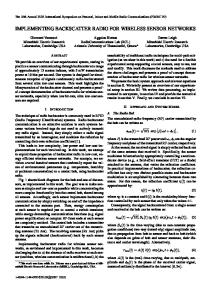
tackle such a privacy breach, the concept of aggregate location information, that is, a collection of location data relating to a group or category of persons from which individual identities have been removed [8], [9], has been suggested as an effective approach to preserve location privacy [6], [8], [9]. Although the counting sensors by nature provide aggregate location information, they would also pose privacy breaches. Figure 1 gives an example of a privacy breach in a location monitoring system with counting sensors. There are 11 counting sensor nodes installed in nine rooms R1 to R9 , and two hallways C1 and C2 (Figure 1a). The nonzero number of persons detected by each sensor node is depicted as a number in parentheses. Figures 1b and 1c

(a) At time ti

(b) At time ti+1

(c) At time ti+2

Fig. 1: A location monitoring system using counting sensors.

2

give the numbers reported by the same set of sensor nodes at two consecutive time instances ti+1 and ti+2 , respectively. If R3 is Alice’s office room, an adversary knows that Alice is in room R3 at time ti . Then the adversary knows that Alice left R3 at time ti+1 and went to C2 by knowing the number of persons detected by the sensor nodes in R3 and C2 . Likewise, the adversary can infer that Alice left C2 at time ti+2 and went to R7 . Such knowledge leakage may lead to several privacy threats. For example, knowing that a person has visited certain clinical rooms may lead to knowing the her health records. Also, knowing that a person has visited a certain bar or restaurant in a mall building may reveal confidential personal information. This paper proposes a privacy-preserving location monitoring system for wireless sensor networks to provide monitoring services. Our system relies on the well established k-anonymity privacy concept, which requires each person is indistinguishable among k persons. In our system, each sensor node blurs its sensing area into a cloaked area, in which at least k persons are residing. Each sensor node reports only aggregate location information, which is in a form of a cloaked area, A, along with the number of persons, N , located in A, where N ≥ k, to the server. It is important to note that the value of k achieves a trade-off between the strictness of privacy protection and the quality of monitoring services. A smaller k indicates less privacy protection, because a smaller cloaked area will be reported from the sensor node; hence better monitoring services. However, a larger k results in a larger cloaked area, which will reduce the quality of monitoring services, but it provides better privacy protection. Our system can avoid the privacy leakage in the example given in Figure 1 by providing low quality location monitoring services for small areas that the adversary could use to track users, while providing high quality services for larger areas. The definition of a small area is relative to the required anonymity level, because our system provides better quality services for the same area if we relax the required anonymity level. Thus the adversary cannot infer the number of persons currently residing in a small area from our system output with any fidelity; therefore the adversary cannot know that Alice is in room R3 . To preserve personal location privacy, we propose two in-network aggregate location anonymization algorithms, namely, resource- and quality-aware algorithms. Both algorithms require the sensor nodes to collaborate with each other to blur their sensing areas into cloaked areas, such that each cloaked area contains at least k persons to constitute a k-anonymous cloaked area. The resource-aware algorithm aims to minimize communication and computational cost, while the quality-aware algorithm aims to minimize the size of the cloaked areas, in order to maximize the accuracy of the aggregate locations reported to the server. In the resource-aware algorithm, each sensor node finds an adequate number of persons, and then it uses a greedy approach to find a

cloaked area. On the other hand, the quality-aware algorithm starts from a cloaked area A, which is computed by the resource-aware algorithm. Then A will be iteratively refined based on extra communication among the sensor nodes until its area reaches the minimal possible size. For both algorithms, the sensor node reports its cloaked area with the number of monitored persons in the area as an aggregate location to the server. Although our system only knows the aggregate location information about the monitored persons, it can still provide monitoring services through answering aggregate queries, for example, “What is the number of persons in a certain area?” To support these monitoring services, we propose a spatial histogram that analyzes the gathered aggregate locations to estimate the distribution of the monitored persons in the system. The estimated distribution is used to answer aggregate queries. We evaluate our system through simulated experiments. The results show that the communication and computational cost of the resource-aware algorithm is lower than the quality-aware algorithm, while the quality-aware algorithm provides more accurate monitoring services (the average accuracy is about 90%) than the resource-aware algorithm (the average accuracy is about 75%). Both algorithms only reveal k-anonymous aggregate location information to the server, but they are suitable for different system settings. The resource-aware algorithm is suitable for the system, where the sensor nodes have scarce communication and computational resources, while the quality-aware algorithm is favorable for the system, where accuracy is the most important factor in monitoring services. The rest of this paper is organized as follows. Our system model is outlined in Section 2. Section 3 presents the resource- and quality-aware location anonymization algorithms. Section 4 describes the aggregate query processing. We describe an attacker model and the experiment setting of our system in Section 5. The experimental results are given in Section 6. Section 7 highlights the related work. Finally, Section 8 concludes the paper.

2

S YSTEM M ODEL

Figure 2 depicts the architecture of our system, where there are three major entities, sensor nodes, server, and system users. We will define the problem addressed by our system, and then describe the detail of each entity and the privacy model of our system. Problem definition. Given a set of sensor nodes s1 , s2 , . . . , sn with sensing areas a1 , a2 , . . . , an , respectively, a set of moving objects o1 , o2 , . . . , om , and a required anonymity level k, (1) we find an aggregate location for each sensor node si in a form of Ri = (Areai , Ni ), where Areai is a rectangular area containing the sensing area of a set of sensor nodes Si and Ni is the number of objects residing in the sensing areas of the sensor nodes in Si , such that Ni ≥ k, Ni = | ∪sj ∈Si Oj | ≥ k, Oj = {ol |ol ∈ aj }, 1 ≤ i ≤ n, and 1 ≤ l ≤ m; and (2) we

3

Fig. 2: System architecture.

build a spatial histogram to answer an aggregate query Q that asks about the number of objects in a certain area Q.Area based on the aggregate locations reported from the sensor nodes. Sensor nodes. Each sensor node is responsible for determining the number of objects in its sensing area, blurring its sensing area into a cloaked area A, which includes at least k objects, and reporting A with the number of objects located in A as aggregate location information to the server. We do not have any assumption about the network topology, as our system only requires a communication path from each sensor node to the server through a distributed tree [10]. Each sensor node is also aware of its location and sensing area. Server. The server is responsible for collecting the aggregate locations reported from the sensor nodes, using a spatial histogram to estimate the distribution of the monitored objects, and answering range queries based on the estimated object distribution. Furthermore, the administrator can change the anonymized level k of the system at anytime by disseminating a message with a new value of k to all the sensor nodes. System users. Authenticated administrators and users can issue range queries to our system through either the server or the sensor nodes, as depicted in Figure 2. The server uses the spatial histogram to answer their queries. Privacy model. In our system, the sensor nodes constitute a trusted zone, where they behave as defined in our algorithm and communicate with each other through a secure network channel to avoid internal network attacks, for example, eavesdropping, traffic analysis, and malicious nodes [6], [11]. Since establishing such a secure network channel has been studied in the literature [6], [11], the discussion of how to get this network channel is beyond the scope of this paper. However, the solutions that have been used in previous works can be applied to our system. Our system also provides anonymous communication between the sensor nodes and the server by employing existing anonymous communication techniques [12], [13]. Thus given an aggregate location R, the server only knows that the sender of R is one of the sensor nodes within R. Furthermore, only authenticated administrators can change the k-anonymity level and the spatial histogram size. In emergency cases, the administrators can set the k-anonymity level to a small value

to get more accurate aggregate locations from the sensor nodes, or even set it to zero to disable our algorithm to get the original readings from the sensor nodes, in order to get the best services from the system. Since the server and the system user are outside the trusted zone, they are untrusted. We now discuss the privacy threat in existing location monitoring systems. In an identity-sensor location monitoring system, since each sensor node reports the exact location information of each monitored object to the server, the adversary can pinpoint each object’s exact location. On the other hand, in a counting-sensor location monitoring system, each sensor node reports the number of objects in its sensing area to the server. The adversary can map the monitored areas of the sensor nodes to the system layout. If the object count of a monitored area is very small or equal to one, the adversary can infer the identity of the monitored objects based on the mapped monitored area, for example, Alice is in her office room at time instance ti in Figure 1. Since our system only allows each sensor node to report a k-anonymous aggregate location to the server, the adversary cannot infer an object’s exact location with any fidelity. The larger the anonymity level, k, the more difficult for the adversary to infer the object’s exact location. With the k-anonymized aggregate locations reported from the sensor nodes, the underlying spatial histogram at the server provides low quality location monitoring services for a small area, and better quality services for larger areas. This is a nice privacy-preserving feature, because the object count of a small area is more likely to reveal personal location information. The definition of a small area is relative to the required anonymity level, because our system provides lower quality services for the same area if the anonymized level gets stricter. We will also describe an attack model, where we stimulate an attacker that could be a system user or the server attempting to infer the object count of a particular sensor node in Section 5.1. We evaluate our system’s resilience to the attack model and its privacy protection in Section 6.

3

L OCATION A NONYMIZATION A LGORITHMS

In this section, we present our in-network resource- and quality-aware location anonymization algorithms that is periodically executed by the sensor nodes to report their k-anonymous aggregate locations to the server for every reporting period. 3.1 The Resource-Aware Algorithm Algorithm 1 outlines the resource-aware location anonymization algorithm. Figure 3 gives an example to illustrate the resource-aware algorithm, where there are seven sensor nodes, A to G, and the required anonymity level is five, k = 5. The dotted circles represent the sensing area of the sensor nodes, and a line between two sensor nodes indicates that these two sensor nodes

4

(a) PeerLists after the first broadcast

(b) Rebroadcast from sensor node F

(c) Resource-aware cloaked area of sensor node A

Fig. 3: The resource-aware location anonymization algorithm (k = 5). can communicate directly with each other. In general, the algorithm has three steps. Step 1: The broadcast step. The objective of this step is to guarantee that each sensor node knows an adequate number of objects to compute a cloaked area. To reduce communication cost, this step relies on a heuristic that a sensor node only forwards its received messages to its neighbors when some of them have not yet found an adequate number of objects. In this step, after each sensor node m initializes an empty list PeerList (Line 2 in Algorithm 1), m sends a message with its identity m.ID, sensing area m.Area, and the number of objects located in its sensing area m.Count, to its neighbors (Line 3). When m receives a message from a peer p, i.e., (p.ID, p.Area, p.Count), m stores the message in its PeerList (Line 5). Whenever m finds an adequate number of objects, m sends a notification message to its neighbors (Line 7). If m has not received the notification message from all its neighbors, some neighbor has not found an adequate number of objects; therefore m forwards the received message to its neighbors (Line 10). Figures 3a and 3b illustrate the broadcast step. When a reporting period starts, each sensor node sends a message with its identity, sensing area, and the number of objects located in its sensing area to its neighbors. After the first broadcast, sensor nodes A to F have found an adequate number of objects (represented by black circles), as depicted in Figure 3a. Thus sensor nodes A to F send a notification message to their neighbors. Since sensor node F has not received a notification message from its neighbor G, F forwards its received messages, which include the information about sensor nodes D and E, to G (Figures 3b). Finally, sensor node G has found an adequate number of objects, so it sends a notification message to its neighbor, F . As all the sensor nodes have found an adequate number of objects, they proceed to the next step. Step 2: The cloaked area step. The basic idea of this step is that each sensor node blurs its sensing area into a cloaked area that includes at least k objects, in order to satisfy the k-anonymity privacy requirement. To minimize computational cost, this step uses a greedy

Algorithm 1 Resource-aware location anonymization 1: function R ESOURCE AWARE (Integer k, Sensor m, List R) 2: PeerList ← {∅} // Step 1: The broadcast step 3: Send a message with m’s identity m.ID, sensing area m.Area, and object count m.Count to m’s neighbor peers 4: if Receive a message from a peer p, i.e., (p.ID, p.Area, p.count) then 5: Add the message to PeerList 6: if m has found an adequate number of objects then 7: Send a notification message to m’s neighbors 8: end if 9: if Some m’s neighbor has not found an adequate number of objects then 10: Forward the message to m’s neighbors 11: end if 12: end if // Step 2: The cloaked area step 13: S ← {m} 14: Compute a score for each peer in PeerList 15: Repeatedly select the peer with the highest score from PeerList to S until the total number of objects in S is at least k 16: Area ← a minimum bounding rectangle of the senor nodes in S 17: N ← the total number of objects in S // Step 3: The validation step 18: if No containment relationship with Area and R ∈ R then 19: Send (Area, N ) to the peers within Area and the server 20: else if m’s sensing area is contained by some R ∈ R then 21: Randomly select a R0 ∈ R such that R0 .Area contains m’s sensing area 22: Send R0 to the peers within R0 .Area and the server 23: else 24: Send Area with a cloaked N to the peers within Area and the server 25: end if

approach to find a cloaked area based on the information stored in PeerList. For each sensor node m, m initializes a set S = {m}, and then determines a score for each peer in its PeerList (Lines 13 to 14 in Algorithm 1). The score is defined as a ratio of the object count of the peer to the Euclidean distance between the peer and m. The idea behind the score is to select a set of peers from PeerList to S to form a cloaked area that includes at least k objects and has an area as small as possible. Then we repeatedly select the peer with the highest score from the PeerList to S until S contains at least k objects (Line 15). Finally, m determines the cloaked area (Area) that is a minimum bounding rectangle (MBR) that covers the sensing area of the sensor nodes in S, and the total number of objects in S (N ) (Lines 16 to 17). An MBR is a rectangle with the minimum area (which is parallel to the axes) that completely contains all desired regions, as illustrated in Figure 3c, where the dotted rectangle is the MBR of the sensing area of sensor

5

nodes A and B. The major reasons of our algorithms aligning with MBRs rather than other polygons are that the concept of MBRs have been widely adopted by existing query processing algorithms and most database management systems have the ability to manipulate MBRs efficiently. Figure 3c illustrates the cloaked area step. The PeerList of sensor node A contains the information of three peers, B, D, and E. The object count of sensor nodes B, D, and E is 3, 1, and 2, respectively. We assume that the distance from sensor node A to sensor nodes B, D, and E is 17, 18, and 16, respectively. The score of B, D, and E is 3/17 = 0.18, 1/18 = 0.06, and 2/16 = 0.13, respectively. Since B has the highest score, we select B. The sum of the object counts of A and B is six which is larger than the required anonymity level k = 5, so we return the MBR of the sensing area of the sensor nodes in S, i.e., A and B, as the resource-aware cloaked area of A, which is represented by a dotted rectangle. Step 3: The validation step. The objective of this step is to avoid reporting aggregate locations with a containment relationship to the server. Let Ri and Rj be two aggregate locations reported from sensor nodes i and j, respectively. If Ri ’s monitored area is included in Rj ’s monitored area, Ri .Area ⊂ Rj .Area or Rj .Area ⊂ Ri .Area, they have a containment relationship. We do not allow the sensor nodes to report their aggregate locations with the containment relationship to the server, because combining these aggregate locations may pose privacy leakage. For example, if Ri .Area ⊂ Rj .Area and Ri .Area 6= Rj .Area, an adversary can infer that the number of objects residing in the non-overlapping area, Rj .Area − Ri .Area, is Rj .N − Ri .N . In case that Rj .N − Ri .N < k, the adversary knows that the number of objects in the non-overlapping is less than k, which violates the k-anonymity privacy requirement. As this step ensures that no aggregate location with the containment relationship is reported to the server, the adversary cannot obtain any deterministic information from the aggregate locations. In this step, each sensor node m maintains a list R to store the aggregate locations sent by other peers. When a reporting period starts, m nullifies R. After m finds its aggregate location Rm , m checks the containment relationship between Rm and the aggregate locations stored in R. If there is no containment relationship between Rm and the aggregate locations in R, m sends Rm to the peers within Rm .Area and the server (Line 19 in Algorithm 1). Otherwise, m randomly selects an aggregate location Rp from the set of aggregate locations in R that contain m’s sensing area, and m sends Rp to the peers within Rp .Area and the server (Lines 21 to 22). In case that no aggregate location in R contains m’s sensing area, we find a set of aggregate locations in R that are contained by Rm , R0 , and N 0 is the number of monitored persons in Rm that is not covered by any aggregate location in R0 . If N 0 ≥ k, the containment relationship does not violate the k-anonymity privacy requirement;

Algorithm 2 Quality-aware location anonymization 1: function Q UALITYAWARE (Integer k, Sensor m, Set init solution, List R) 2: current min cloaked area ← init solution // Step 1: The search space step 3: Determine a search space S based on init solution 4: Collect the information of the peers located in S // Step 2: The minimal cloaked area step 5: Add each peer located in S to C[1] as an item 6: Add m to each itemset in C[1] as the first item 7: for i = 1; i ≤ 4; i ++ do 8: for each itemset X = {a1 , . . . , ai+1 } in C[i] do 9: if Area(M BR(X)) < Area(current min cloaked area) then 10: if N (M BR(X)) ≥ k then 11: current min cloaked area ← {X} 12: Remove X from C[i] 13: end if 14: else 15: Remove X from C[i] 16: end if 17: end for 18: if i < 4 then 19: for each itemset pair X={x1 ,. . . ,xi+1 }, Y ={y1 ,. . . ,yi+1 } in C[i] do 20: if x1 = y1 , . . . , xi = yi and xi+1 6= yi+1 then 21: Add an itemset {x1 , . . . , xi+1 , yi+1 } to C[i + 1] 22: end if 23: end for 24: end if 25: end for 26: Area ← a minimum bounding rectangle of current min cloaked area 27: N ← the total number of objects in current min cloaked area // Step 3: The validation step 28: Lines 18 to 25 in Algorithm 1

therefore m sends Rm to the peers within Rm .Area and the server. However, if N 0 < k, m cloaks the number of monitored persons of Rm , Rm .N , by increasing it by an integer uniformly selected between k and 2k, and sends Rm to the peers within Rm .Area and the server (Line 24). Since the server receives an aggregate location from each sensor node for every reporting period, it cannot tell whether any containment relationship takes place among the actual aggregate locations of the sensor nodes. 3.2 The Quality-Aware Algorithm Algorithm 2 outlines the quality-aware algorithm that takes the cloaked area computed by the resource-aware algorithm as an initial solution, and then refines it until the cloaked area reaches the minimal possible area, which still satisfies the k-anonymity privacy requirement, based on extra communication between other peers. The quality-aware algorithm initializes a variable current minimal cloaked area by the input initial solution (Line 2 in Algorithm 2). When the algorithm terminates, the current minimal cloaked area contains the set of sensor nodes that constitutes the minimal cloaked area. In general, the algorithm has three steps. Step 1: The search space step. Since a typical sensor network has a large number of sensor nodes, it is too costly for a sensor node m to gather the information of all the sensor nodes to compute its minimal cloaked area. To reduce communication and computational cost, m determines a search space, S, based on the input initial solution, which is the cloaked area computed by the resource-aware algorithm, such that the sensor nodes outside S cannot be part of the minimal cloaked

6

(a) The MBR of A’s sensing area

(b) The extended MBR1 of the edge e1 (c) The extended MBRi (1 ≤ i ≤ 4)

(d) The search space S

Fig. 4: The search space S of sensor node A. area (Line 3 in Algorithm 2). We will describe how to determine S based on the example given in Figure 4. Thus gathering the information of the peers residing in S is enough for m to compute the minimal cloaked area for m (Line 4). Figure 4 illustrates the search space step, in which we compute S for sensor node A. Let Area be the area of the input initial solution. We assume that Area = 1000. We determine S for A by two steps. (1) We find the minimum bounding rectangle (MBR) of the sensing area of A. It is important to note that the sensing area can be in any polygon or irregular shape. In Figure 4a, the MBR of the sensing area of A is represented by a dotted rectangle, where the edges of the MBR are labeled by e1 to e4 . (2) For each edge ei of the MBR, we compute an MBRi by extending the opposite edge such that the area of the extended MBRi is equal to Area. S is the MBR of the four extended MBRi . Figure 4b depicts the extended MBR1 of the edge e1 by extending the opposite edge e3 , where MBR1 .x is the length of MBR1 , MBR1 .y = Area/MBR1 .x and Area = 1000. Figure 4c shows the four extended MBRs, MBR1 to MBR4 , which are represented by dotted rectangles. The MBR of the four extended MBRs constitutes S, which is represented by a rectangle (Figure 4d). Finally, the sensor node only needs the information of the peers within S. Step 2: The minimal cloaked area step. This step takes a set of peers residing in the search space, S, as an input and computes the minimal cloaked area for the sensor node m. Although the search space step already prunes the entire system space into S, exhaustively searching the minimal cloaked area among the peers residing in S, which needs to search all the possible combinations of these peers, could still be costly. Thus we propose two optimization techniques to reduce computational cost. The basic idea of the first optimization technique is that we do not need to examine all the combinations of the peers in S; instead, we only need to consider the combinations of at most four peers. The rationale behind this optimization is that an MBR is defined by at most four sensor nodes because at most two sensor

Fig. 5: The lattice structure of a set of four items.

nodes define the width of the MBR (parallel to the x-axis) while at most two other sensor nodes define the height of the MBR (parallel to the y-axis). Thus this optimization mainly reduces computational cost by reducing the number of MBR computations among the peers in S. The correctness of this optimization technique will be discussed in Section 3.2.2. The second optimization technique has two properties, lattice structure and monotonicity property. We first describe these two properties, and then present a progressive refinement approach for finding a minimal cloaked area. A. Lattice structure. In a lattice structure, a data set that contains n items can generate 2n−1 itemsets excluding a null set. In the sequel, since the null set is meaningless to our problem, it will be neglected. Figure 5 shows the lattice structure of a set of four items S = {s1 , s2 , s3 , s4 }, where each black line between two itemsets indicates that an itemset at a lower level is a subset of an itemset at a higher level. For our problem, given a set of sensor nodes S = {s1 , s2 , . . . , sn }, all the possible combinations of these sensor nodes are the non-empty subsets of S; thus we can use a lattice structure to generate the combinations of the sensor nodes in S. In the lattice structure, since each itemset at level i has i items in S, each combination at the lowest level, level 1, contains a distinct item in S; therefore there are n itemsets at the lowest level. We generate the lattice structure from the

7

(a) The full lattice structure

(b) Pruning itemset {A, B}

(c) Pruning itemset {A, D}

(d) The minimal cloaked area

Fig. 6: The quality-aware cloaked area of sensor node A. lowest level based on a simple generation rule: given two sorted itemsets X = {x1 , . . . , xi } and Y = {y1 , . . . , yi } in increasing order, where each itemset has i items (1 ≤ i < n), if all item pairs but the last one in X and Y are the same, x1 = y1 , x2 = y2 , . . ., xi−1 = yi−1 , and xi 6= yi , we generate a new itemset with i + 1 items, {x1 , . . . , xi , yi }. In the example, we use bold lines to illustrate the construction of the lattice structure based on the generation rule. For example, the itemset {s1 , s2 , s3 , s4 } at level 4 is combined by the itemsets {s1 , s2 , s3 } and {s1 , s2 , s4 } at level 3, so there is a bold line from {s1 , s2 , s3 , s4 } to {s1 , s2 , s3 } and another one to {s1 , s2 , s4 }. B. Monotonicity property. Let S be a set of items, and P be the power set of S, 2S . The monotonicity property of a function f indicates that if X is a subset of Y , then f (X) must not exceed f (Y ), i.e., ∀X, Y ∈ P : (X ⊆ Y ) → f (X) ≤ f (Y ). For our problem, the MBR of a set of sensor nodes S has the monotonicity property, because adding sensor nodes to S must not decrease the area of the MBR of S or the number of objects within the MBR of S. Let Area(M BR(X)) and N (M BR(X)) be two functions that return the area of the MBR of an itemset X and the number of monitored objects located in the MBR, respectively. Thus, given two itemsets X and Y , if X ⊆ Y , then Area(M BR(X)) ≤ Area(M BR(Y )) and N (M BR(X)) ≤ N (M BR(Y )). By this property, we propose two pruning conditions in the lattice structure. (1) If a combination C gives the current minimal cloaked area, other combinations that contain C at the higher levels of the lattice structure should be pruned. This is because the monotonicity property indicates that the pruned combinations cannot constitute a cloaked area smaller than the current minimal cloaked area. (2) Similarly, if a combination C constitutes a cloaked area that is the same or larger than the current minimal cloaked area, other combinations that contain C at the higher levels of the lattice structure should be pruned. C. Progressive refinement. Since the monotonicity property shows that we would not need to generate a complete lattice structure to compute a minimal cloaked area, we generate the lattice structure of the peers in the search space, S, progressively from the lowest level of the lattice structure to its higher levels, in order to minimize the

computational and storage overhead. To compute the minimal cloaked area for the sensor node m, we first generate an itemset for each peer in S at the lowest level of the lattice structure, C[1] (Line 5 in Algorithm 2). To accommodate with our problem, we add m to each itemset in C[1] as the first item (Line 6). Such accommodation does not affect the generation of the lattice structure, but each itemset has an extra item, m. For each itemset X in C[1], we determine the MBR of X, M BR(X). If the area of M BR(X) is less than the current minimal cloaked area and the total number of objects in M BR(X) is at least k, we set X to the current minimal cloaked area, and remove X from C[1] based on the first pruning condition of the monotonicity property (Lines 11 to 12). However, if the area of M BR(X) is equal to or larger than the area of the current minimal cloaked area, we also remove X from C[1] based on the second pruning condition of the monotonicity property (Line 15). Then we generate the itemsets, where each itemset contains two items, at the second lowest level of the lattice structure, C[2], based on the remaining itemsets in C[1] based on the generation rule of the lattice structure. We repeat this procedure until we produce the itemsets at the highest level of the lattice structure, C[4], or all the itemsets at the current level are pruned (Lines 19 to 23). After we examine all non-pruned itemsets in the lattice structure, the current minimal cloaked area stores the combination giving the minimal cloaked area (Lines 26 to 27). Figure 6 illustrates the minimal cloaked area step that computes the minimal cloaked area for sensor node A. The set of peers residing in the search space is S = {B, D, E}. We assume that the area of the MBR of {A, B}, {A, D}, and {A, E} is 1000, 1200, and 900, respectively. The number of objects residing in the MBR of {A, B}, {A, D}, and {A, E} is six, four, and five, respectively, as depicted in Figure 3. Figure 6a depicts the full lattice structure of S where A is added to each itemset as the first item. Initially, the current minimal cloaked area is set to the initial solution, which is the MBR of {A, B} ’computed by the resource-aware algorithm. The area of the MBR of {A, B}, Area(M BR({A, B})), is 1000 and the total number of monitored objects in M BR({A, B}), N (M BR({A, B})), is six. It is important to note that

8

the progressive refinement approach may not require our algorithm to compute the full lattice structure. As depicted in Figure 6b, we construct the lowest level of the lattice structure, where each itemset contains a peer in S. Since the area of M BR({A, B}) is the current minimal cloaked area, we remove {A, B} from the lattice structure; hence the itemsets at the higher levels that contain {A, B}, {A, B, D}, {A, B, E}, and {A, B, D, E} (enclosed by a dotted oval), will not be considered by the algorithm. Then, we consider the next itemset {A, D}. Since the area of M BR({A, D}) is larger than the current minimal cloaked area, this itemset is removed from the lattice structure. After pruning {A, D}, the itemsets at the higher levels that contain {A, D}, {A, D, E} (enclosed by a dotted oval), will not be considered (Figure 6c). We can see that all itemsets beyond the lowest level of the lattice structure will not be considered by the algorithm. Finally, we consider the last itemset {A, E}. Since the area of M BR({A, E}) is less than current minimal cloaked area and the total number of monitored objects in M BR({A, E}) is k = 5, we set {A, E} to the current minimal cloaked area (Figure 6d). As the algorithm cannot generate any itemsets at the higher level of the lattice structure, it terminates. Thus the minimal cloaked area is the MBR of sensor nodes A and E, and the number of monitored objects in this area is five. Step 3: The validation step. This step is exactly the same as in the resource-aware algorithm (Section 3.1). 3.2.1 Analysis A brute-force approach of finding the minimal cloaked area of a sensor node has to examine all the combinations of its peers. Let N be the number of sensor nodes in the system. Since each sensor node has N − 1 peers, PN −1 N −1 we have to consider = 2N −1 − 1 MBRs i=1 Ci to find the minimal cloaked area. In our algorithm, the search space step determines a search space, S, and prunes the peers outside S. Let M be the number of peers in S, where M ≤ N − 1. Thus the computational PM cost is reduced to i=1 CiM = 2M − 1. In the minimal cloaked area step, the first optimization technique indicates that an MBR can be defined by at most four peers. As we need to consider the combinations of at most peers, the computational cost is reduced to P4 four M C = (M 4 − 2M 3 + 11M 2 + 14M )/24 = O(M 4 ). i=1 i Furthermore, the second optimization technique uses the monotonicity property to prune the combinations, which cannot give the minimal cloaked area. In our example, the brute-force approach considers all the combinations of six peers; hence this approach computes 26 − 1 = 63 MBRs to find the minimal cloaked area of sensor node A. In our algorithm, the search space step reduces the entire space into S, which contains only three peers; hence this step needs to compute 23 − 1 = 7 MBRs. After examining the three itemsets at the lowest level of the lattice structure, all other itemsets at the higher levels are pruned. Thus the progressive refinement approach considers only three combinations. Therefore our

algorithm reduces over 95% computational cost of the brute-force approach, as it reduces the number of MBR computations from 63 to 3. 3.2.2 Proof of Correctness In this section, we show the correctness of the qualityaware location anonymization algorithm. Theorem 1: Given a resource-aware cloaked area of size Area of a sensor node s, a search space, S, computed by the quality-aware algorithm contains the minimal cloaked area. Proof: Let X be the minimal cloaked area of size equal to or less than Area. We know that X must totally cover the sensing area of s. Suppose X is not totally covered by S, X must contain at least one extended MBR, MBRi , where 1 ≤ i ≤ 4 (Figure 4c). This means that the area of X is larger than the area of an extended MBR, Area. This contradicts to the assumption that X is the minimal cloaked area; thus X is included in S. Theorem 2: A minimum bounding rectangle (MBR) can be defined by at most four sensor nodes. Proof: By definition, given an MBR, each edge of the MBR touches the sensing area of some sensor node. In an extreme case, there is a distinct sensor node touching each edge of the MBR but not other edges. The MBR is defined by four sensor nodes, which touch different edges of the MBR. For any edge e of the MBR, if multiple sensor nodes touch e but not other edges, we can simply pick one of these sensor nodes, because any one of these sensor nodes gives the same e. Thus an MBR is defined by at most four sensor nodes.

4 S PATIAL H ISTOGRAM In this section, we present a spatial histogram that is embedded inside the server to estimate the distribution of the monitored objects based on the aggregate locations reported from the sensor nodes. Our spatial histogram is represented by a two-dimensional array that models a grid structure G of NR rows and NC columns; hence, the system space is divided into NR × NC disjoint equalsized grid cells. In each grid cell G(i, j), we maintain a float value that acts as an estimator H[i, j] (1 ≤ i ≤ NC , 1 ≤ j ≤ NR ) of the number of objects within its area. We assume that the system has the ability to know the total number of moving objects M in the system. The value of M will be used to initialize the spatial histogram. In practice, M can be computed online for both indoor and outdoor dynamic environments. For the indoor environment, the sensor nodes can be deployed at each entrance and exit to count the number of users entering or leaving the system [4], [5]. For the outdoor environment, the sensor nodes have been already used to count the number of people in a predefined area [3]. We use the spatial histogram to provide approximate location monitoring services. The accuracy of the spatial histogram that indicates the utility of our privacypreserving location monitoring system will be evaluated in Section 6.

9

Algorithm 3 Spatial histogram maintenance

5.1 Attacker Model

1: function H ISTOGRAM M AINTENANCE (AggregateLocationSet R) 2: for each aggregate location R ∈ R do 3: if there is an existing partition P = {R1 , . . . , R|P | } such that R.Area∩ Rk .Area = ∅ for every Rk ∈ P then 4: Add R to P 5: else 6: Create a new partition for R 7: end if 8: end for 9: for each partition P do 10: for each aggregate P location Rk ∈ P do b← 11: R k .N H[i, j]

To evaluate the privacy protection of our system, we simulate an attacker attempting to infer the number of objects residing in a sensor node’s sensing area. We will analyze the evaluation result in Section 6.1. The key idea of the attacker model is that if the attacker cannot infer the exact object count of the sensor node from our system output, the attacker cannot infer the location information corresponding to an individual object. We consider the worst-case scenario where the attacker has the background knowledge about the system, i.e., the map layout of the system, the location of each sensor node, the sensing area of each sensor node, the total number of objects currently residing in the system, and the aggregate locations reported from the sensor nodes. In general, the attacker model is defined as: Given an area A (that corresponds to the monitored area of a sensor node) and a set of aggregate locations R = {R1 , R2 , . . . , R|R| } overlapping with A, the attacker estimates the number of persons within A. Since the validation step in our location anonymization algorithms does not allow the aggregate locations with the containment relationship to be reported to the server, no aggregate location is included in other aggregate locations in R. Without loss of generality, we use the Poisson distribution as a concrete exemplary distribution for the attacker model [14]. Under the Poisson distribution, objects are uniformly distributed in an area within intensity of λ. The probability of n distinct objects in a region S of size −λs n s is: P (N (S) = n) = e n!(λs) , where λ is computed as the number of objects in the system divided by the area of the system. Suppose that the object count of each aggregate location Ri is ni , where 1 ≤ i ≤ |R|, and the aggregate locations in R and A constitute m non-overlapping subregions Sj , where 1 ≤ j ≤ m; hence, N (Ri ) = P Sj ∈Ri N (Sj ) = ni . Each subregion must either intersect or not intersect A, and it intersects one or more aggregate locations. If a subregion Sk intersects A, but none of the aggregate locations in R, then N (Sk ) = 0. The probability mass function of the number of distinct objects in A being equal to na , N = na , given the aggregate locations in R can be expressed as follows:

12: 13: 14: 15:

G[i,j]∈Rk .Area

For every cell G(i, j) ∈ Rk .Area, H[i, j] ← end for P.Area ← R1 .Area ∪ . . . ∪ R|P | .Area For every cell G(i, j) ∈ /P P.Area,

H[i, j] = H[i, j] + 16: end for

Rk .N No. of cells within Rk .Area

b

Rk .N −Rk .N Rk ∈P No. of cells outside P.Area

Algorithm 3 outlines our spatial histogram approach. Initially, we assume that the objects are evenly distributed in the system, so the estimated number of objects within each grid cell is H[i, j] = M/(NR × NC ). The input of the histogram is a set of aggregate locations R reported from the sensor nodes. Each aggregate location R in R contains a cloaked area, R.Area, and the number of monitored objects within R.Area, R.N . First, the aggregate locations in R are grouped into the same partition P = {R1 , R2 , . . . , R|P | } if their cloaked areas are not overlapping with each other, which means that for every pair of aggregate locations Ri and Rj in P , Ri .Area ∩ Rj .Area = ∅ (Lines 2 to 8. Then, for each partition P , we update its entire set of aggregate locations to the spatial histogram at the same time. For each aggregate location R in P , we record the estimation error, which is the difference between the sum of the b , and R.N , and then R.N estimators within R.Area, R.N is uniformly distributed among the estimators within R.Area; hence, each estimator within R.Area is set to R.N divided by the total number of grid cells within R.Area (Lines 10 to 13). After processing all the aggregate locations in P , we sum up the estimation error of P|P | b − Rk .N , that each aggregate location in P , k=1 Rk .N is uniformly distributed among the estimators outside P.Area, where P.Area is the area covered by some aggregate location in P , P.Area = ∪Rk ∈P Rk .Area (Line 15). Formally, for each partition P that contains |P | aggregate locations Rk (1 ≤ k ≤ |P |), every estimator in the histogram is updated as follows:  Rk .N for G(i, j) ∈ Rk .Area  No. of cells within Rk .Area , P|P | H[i, j] = b k .N  Rk .N−R H[i, j] + No. ofk=1 / P.Area cells outside P.Area , for G(i, j) ∈

5

S YSTEM E VALUATION

In this section, we discuss an attacker model, the experiment setting of our privacy-preserving location monitoring system in a wireless sensor network, and the performance metrics.

P (N = na |N (R1 ) = n1 , . . . , N (R|R| ) = n|R| ) P (N = na , N (R1 ) = n1 , . . . , N (R|R| ) = n|R| ) = P (N (R1 ) = n1 , . . . , N (R|R| ) = n|R| ) P i i i Vi ∈(VS ∩VA ) < v1 , v2 , . . . , vm > = P , j j j Vj ∈VS < v1 , v2 , . . . , vm >

(1)

where the notation V =< v1 , v2 , . . . , vm > represents the joint probability that there are vi objects in a subregion Si (1 ≤ i ≤ m); the joint probability is computed as Q 1≤i≤m P (N (Si ) = vi ). The lower and upper bounds of vi (denoted as LB(vi ) and U B(vi ), respectively) are zero and the minimum nj of the aggregate locations inter-

10

Default Value 200 × 200 [0.001, 0.032] 5,000 20 [0,5]

0.6

Range 502 to 2502 0.001 to 0.256 2,000 to 10,000 10 to 30 [0,5] to [0,30]

0.7

Resource-Aware Quality-Aware

0.5

0.5

0.4

0.4

0.3

0.3

0.2

0.2

0.1 0

secting Si , respectively. Thus, the possible value of vi is within a range of [0, minRj ∩Si 6=∅∧1≤i≤m∧1≤j≤|R| (nj )]. VS is the set of < v1 , v2 , . . . , vP to the m > that is a solution P following equations: V : v = n , S 1 Si ∈R1 i Si ∈R2 vi = P n2 , . . . , Si ∈R|R| vi = n|R| , where vi ≥ 0 for 1 ≤ i ≤ m. VA is the set of < v1 , vP 2 , . . . , vm > that satisfies the following equation: VA : 1≤i≤m vi = na . The attacker uses an exhaustive approach to find all possible solutions to VS , in order to compute the expected value E(N ) of Equation 1 as the estimated value Q of na . The complexity of computing E(N ) is O( 1≤i≤m U B(vi )). Since the complexity of the attacker model is an exponential function of m and m would be much larger than |R|, such exponential complexity makes it prohibitive for the attacker model to be used to provide online location monitoring services; and therefore, we use our spatial histogram to provide online services in the experiments. We will evaluate the resilience of our system to the attacker model in Section 6.1. 5.2 Simulation Settings In all experiments, we simulate 30 × 30 sensor nodes that are uniformly distributed in a 600 × 600 system space. Each sensor node is responsible for monitoring a 20 × 20 space. We generate a set of moving objects that freely roam around the system space. Unless mentioned otherwise, the experiments consider 5,000 moving objects that move at a random speed within a range of [0, 5] space unit(s) per time unit, and the required anonymity level is k = 20. The spatial histogram contains NR ×NC = 200×200 grid cells, and we issue 1,000 range queries whose query region size is specified by a ratio of the query region area to the system area, that is, a query region size ratio. The default query region size ratio is uniformly selected within a range of [0.001, 0.032]. Table 1 gives a summary of the parameter settings. 5.3 Performance Metrics We evaluate our system in terms of five performance metrics. (1) Attack model error. This metric measures the resilience of our system to the attacker model by the b relative error between the estimated number of objects N in a sensor node’s sensing area and the actual one N . The b | error is measured as |N−N . When N = 0, we consider N b as the error. (2) Communication cost. We measure the N communication cost of our location anonymization algorithms in terms of the average number of bytes sent by

Resource-Aware Quality-Aware

0.6

Attack Model Error

Description Histogram size (NR × NC ) Query region size ratio Number of moving objects k-anonymity level Object mobility speed

0.7

Attack Model Error

TABLE 1: Parameter settings

0.1 10

15 20 25 Anonymity Levels

30

(a) Anonymity levels

0

2 4 6 8 10 Number of Objects (in thousands)

(b) Number of objects

Fig. 7: Attacker model error. each sensor node per reporting period. This metric also indicates the network traffic and the power consumption of the sensor nodes. (3) Cloaked area size. This metric measures the quality of the aggregate locations reported by the sensor nodes. The smaller the cloaked area, the better the accuracy of the aggregate location is. (4) Computational cost. We measure the computational cost of our location anonymization algorithms in terms of the average number of minimum bounding rectangle (MBR) computations that are needed to determine a resource- or quality-aware cloaked area. We compare our algorithms with a basic approach that computes the MBR for each combination of the peers in the required search space to find the minimal cloaked area. The basic approach does not employ any optimization techniques proposed for our quality-aware algorithm. (5) Query error. This metric measures the utility of our system, in terms of c, which is the relative error between the query answer M the estimated number of objects within the query region based on a spatial histogram, and the actual answer b −M | M , respectively. The error is measured as |MM . When c as the error. M = 0, we consider M

6

E XPERIMENTAL R ESULTS

AND

A NALYSIS

In this section, we show and analyze the experimental results with respect to the privacy protection and the quality of location monitoring services of our system. 6.1 Anonymization Strength Figure 7 depicts the resilience of our system to the attacker model with respect to the anonymity level and the number of objects. In the figure, the performance of the resource- and quality-aware algorithms is represented by black and gray bars, respectively. Figure 7a depicts that the stricter the anonymity level, the larger the attacker model error will be encountered by an adversary. When the anonymity level gets stricter, our algorithms generate larger cloaked areas, which reduce the accuracy of the aggregate locations reported to the server. Figure 7b shows that the attacker model error reduces, as the number of objects gets larger. This is because when there are more objects, our algorithms generate smaller

11

0.8

k=10 k=15 k=20 k=25 k=30

Query Answer Error

0.7 0.6 0.5 0.4 0.3 0.2 0.1 0

0.001

0.002

0.004

0.008 0.016 0.032 Query Region Size Ratio

0.064

0.128

0.256

(a) Resource-aware algorithm 0.6

Query Answer Error

6.3 Effect of the Number of Objects k=10 k=15 k=20 k=25 k=30

0.5 0.4 0.3 0.2 0.1 0

0.001

0.002

0.004

0.008 0.016 0.032 Query Region Size Ratio

0.064

if its query region size is not larger than 0.016 (it is about 16 sensor nodes’ sensing area). For the qualityaware algorithm, Figure 8b shows that when k = 10, a query region is said to be small if its query region size is not larger than 0.002, while when k = 30, a query region is only considered as small if its query region size is not larger than 0.004. The results also show that the quality-aware algorithm always performs better than the resource-aware algorithm.

0.128

0.256

(b) Quality-aware algorithm

Fig. 8: Query region size. cloaked areas, which increase the accuracy of the aggregate locations reported to the server. It is difficult to set a hard quantitative threshold for the attacker model error. However, it is evident that the adversary cannot infer the number of objects in the sensor node’s sensing area with any fidelity. 6.2 Effect of Query Region Size Figure 8 depicts the privacy protection and the quality of our location monitoring system with respect to increasing the query region size ratio from 0.001 to 0.256, where the query region size ratio is the ratio of the query region area to the system area and the query region size ratio 0.001 corresponds to the size of a sensor node’s sensing area. The results give evidence that our system provides low quality location monitoring services for the range query with a small query region, and better quality services for larger query regions. This is an important feature to protect personal location privacy, because providing the accurate number of objects in a small area could reveal individual location information; therefore an adversary cannot use our system output to track the monitored objects with any fidelity. The definition of a small query region is relative to the required anonymity level k. For example, we want to provide low quality services, such that the query error is at least 0.2, for small query regions. For the resource-aware algorithm, Figure 8a shows that when k = 10, a query region is said to be small if its query region size is not larger than 0.002 (it is about two sensor nodes’ sensing area). However, when k = 30, a query region is only considered as small

Figure 9 depicts the performance of our system with respect to increasing the number of objects from 2,000 to 10,000. Figure 9a shows that when the number of objects increases, the communication cost of the resource-aware algorithm is only slightly affected, but the quality-aware algorithm significantly reduces the communication cost. The broadcast step of the resource-aware algorithm effectively allows each sensor node to find an adequate number of objects to blur its sensing area. When there are more objects, the sensor node finds smaller cloaked areas that satisfy the k-anonymity privacy requirement, as given in Figure 9b. Thus the required search space of a minimal cloaked area computed by the quality-aware algorithm becomes smaller; hence the communication cost of gathering the information of the peers in such a smaller required search space reduces. Likewise, since there are less peers in the smaller required search space as the number of objects increases, finding the minimal cloaked area incurs less minimum bounding rectangle (MBR) computation (Figure 9c). Since our algorithms generate smaller cloaked areas when there are more users, the spatial histogram can gather more accurate aggregate locations to estimate the object distribution; therefore the query answer error reduces (Figure 9d). The result also shows that the quality-aware algorithm always provides better quality services than the resourceaware algorithm. 6.4 Effect of Privacy Requirements Figure 10 depicts the performance of our system with respect to varying the required anonymity level k from 10 to 30. When the k-anonymity privacy requirement gets stricter, the sensor nodes have to enlist more peers for help to blur their sensing areas; therefore the communication cost of our algorithms increases (Figure 10a). To satisfy the stricter anonymity levels, our algorithms generate larger cloaked areas, as depicted in Figure 10b. For the quality-aware algorithm, since there are more peers in the required search space when the input (resourceaware) cloaked area gets larger, the computational cost of computing the minimal cloaked area by the qualityaware algorithm and the basic approach gets worse (Figure 10c). However, the quality-aware algorithm reduces the computational cost of the basic approach by at least four orders of magnitude. Larger cloaked areas give more inaccurate aggregate location information to the

8 7 6 5 4 3

2 4 6 8 10 Number of Objects (in thousands)

2.6

108

Resource-Aware Quality-Aware

2.4 2.2

104

1.6

3

10

1.4

2

10

101

1.2

100

1

(a) Communication cost

5

10

1.8

0.8

6

10

2

0.25

Resource-Aware Quality-Aware Basic

7

10

Query Answer Error

Resource-Aware Quality-Aware

9

No. of MBR Computations

10

Cloaked Area Size (in thousands)

Number of Bytes (in thousands)

12

-1

2 4 6 8 10 Number of Objects (in thousands)

10

(b) Cloaked area size

0.15 0.1 0.05 0

2 4 6 8 10 Number of Objects (in thousands)

Resource-Aware Quality-Aware

0.2

(c) Computational cost

2 4 6 8 10 Number of Objects (in thousands)

(d) Estimation error

Resource-Aware Quality-Aware

11 10 9 8 7 6 5 4 3

10

15 20 25 Anonymity Levels

20

(a) Communication cost

3.5 3

109

Resource-Aware Quality-Aware

108 10

106

2.5

5

10

2

4

10

3

10

1.5

2

10

101

1 0.5

7

0.3

Resource-Aware Quality-Aware Basic

Query Answer Error

12

No. of MBR Computations

13

Cloaked Area Size (in thousands)

Number of Bytes (in thousands)

Fig. 9: Number of objects.

0

10

10

15 20 25 Anonymity Levels

30

(b) Cloaked area size

10-1

10

15 20 25 Anonymity Levels

(c) Computational cost

30

0.25

Resource-Aware Quality-Aware

0.2 0.15 0.1 0.05 0

10

15 20 25 Anonymity Levels

30

(d) Estimation error

Fig. 10: Anonymity levels. system, so the estimation error increases as the required k-anonymity increases (Figure 10d). The quality-aware algorithm provides much better quality location monitoring services than the resource-aware algorithm, when the required anonymity level gets stricter. 6.5 Effect of Mobility Speeds Figure 11 gives the performance of our system with respect to increasing the maximum object mobility speed from [0, 5] and [0, 30]. The results show that increasing the object mobility speed only slightly affects the communication cost and the cloaked area size of our algorithms, as depicted in Figures 11a and 11b, respectively. Since the resource-aware cloaked areas are slightly affected by the mobility speed, the object mobility speed has a very small effect on the required search space computed by the quality-aware algorithm. Thus the computational cost of the quality-aware algorithm is also only slightly affected by the object mobility speed (Figure 11c). Although Figure 11d shows that query answer error gets worse when the objects are moving faster, the query accuracy of the quality-aware algorithm is consistently better than the resource-aware algorithm.

7

R ELATED WORK

Straightforward approaches for preserving users’ location privacy include enforcing privacy policies to restrict the use of collected location information [15], [16] and anonymizing the stored data before any disclosure [17]. However, these approaches fail to prevent

internal data thefts or inadvertent disclosure. Recently, location anonymization techniques have been widely used to anonymize personal location information before any server gathers the location information, in order to preserve personal location privacy in location-based services. These techniques are based on one of the three concepts. (1) False locations. Instead of reporting the monitored object’s exact location, the object reports n different locations, where only one of them is the object’s actual location while the rest are false locations [18]. (2) Spatial cloaking. The spatial cloaking technique blurs a user’s location into a cloaked spatial area that satisfy the user’s specified privacy requirements [19], [20], [21], [22], [23], [24], [25], [26], [27], [28]. (3) Space transformation. This technique transforms the location information of queries and data into another space, where the spatial relationship among the query and data are encoded [29]. Among these three privacy concepts, only the spatial cloaking technique can be applied to our problem. The main reasons for this are that (a) the false location techniques cannot provide high quality monitoring services due to a large amount of false location information; (b) the space transformation techniques cannot provide privacy-preserving monitoring services as it reveals the monitored object’s exact location information to the query issuer; and (c) the spatial cloaking techniques can provide aggregate location information to the server and balance a trade-off between privacy protection and the quality of services by tuning the specified privacy requirements, for example, k-anonymity and minimum area privacy requirements [17], [27]. Thus we adopt the

13

6 4 2

2

8

10

Resource-Aware Quality-Aware Basic

6

10

1.5

4

10

1

102

0.5

100

0

5

10 15 20 25 30 Maximum Mobility Speed

(a) Communication cost

0

5

10 15 20 25 30 Maximum Mobility Speed

5

(b) Cloaked area size

10 15 20 25 30 Maximum Mobility Speed

(c) Computational cost

0.3 Query Answer Error

8

Resource-Aware Quality-Aware

No. of MBR Computations

2.5

Resource-Aware Quality-Aware Cloaked Area Size (K)

Number of Bytes (K)

10

0.25

Resource-Aware Quality-Aware

0.2 0.15 0.1 0.05 0

5

10 15 20 25 30 Maximum Mobility Speed

(d) Estimation error

Fig. 11: Object mobility speeds. spatial cloaking technique to preserve the monitored object’s location privacy in our location monitoring system. In terms of system architecture, existing spatial cloaking techniques can be categorized into centralized [19], [20], [22], [25], [26], [27], [28], distributed [23], [24], and peer-to-peer [21] approaches. In general, the centralized approach suffers from the mentioned internal attacks, while the distributed approach assumes that mobile users communicate with each other through base stations is not applicable to the wireless sensor network. Although the peer-to-peer approach can be applied to the wireless sensor network, the previous work using this approach only focuses on hiding a single user location with no direct applicability to sensor-based location monitoring. Also, the previous peer-to-peer approaches do not consider the quality of cloaked areas and discuss how to provide location monitoring services based on the gathered aggregate location information. In the wireless sensor network, Cricket [2] is the only privacy-aware location system that provides a decentralized positioning service for its users where each user can control whether to reveal her location to the system. However, when many users decide not to reveal their locations, the location monitoring system cannot provide any useful services. This is in contrast to our system that aims to enable the sensor nodes to provide the privacy-preserving aggregate location information of the monitored objects. The closest work to ours is the hierarchical location anonymization algorithm [6] that divides the system space into hierarchical levels based on the physical units, for example, sub-rooms, rooms and floors. If a unit contains at least k users, the algorithm cloaks the subject count by rounding the value to the nearest multiple of k. Otherwise, the algorithm cloaks the location of the physical unit by selecting a suitable space containing at least k users at the higher level of the hierarchy. This work is not applicable to some landscape environments, for example, shopping mall and stadium, and outdoor environments. Our work distinguishes itself from this work, as (1) we do not assume any hierarchical structures, so it can be applied to all kinds of environments, and (2) we consider the problem of how to utilize the anonymized location data to provide privacy-preserving location monitoring ser-

vices while the usability of anonymized location data was not discussed in [6]. Other privacy related works include: anonymous communication that provides anonymous routing between the sender and the receiver [12], source location privacy that hides the sender’s location and identity [13], aggregate data privacy that preserves the privacy of the sensor node’s aggregate readings during transmission [30], data storage privacy that hides the data storage location [31], and query privacy that avoids disclosing the personal interests [32]. However, none of these previous works is applicable to our problem.

8

C ONCLUSION

In this paper, we propose a privacy-preserving location monitoring system for wireless sensor networks. We design two in-network location anonymization algorithms, namely, resource- and quality-aware algorithms, that preserve personal location privacy, while enabling the system to provide location monitoring services. Both algorithms rely on the well established k-anonymity privacy concept that requires a person is indistinguishable among k persons. In our system, sensor nodes execute our location anonymization algorithms to provide kanonymous aggregate locations, in which each aggregate location is a cloaked area A with the number of monitored objects, N , located in A, where N ≥ k, for the system. The resource-aware algorithm aims to minimize communication and computational cost, while the quality-aware algorithm aims to minimize the size of cloaked areas in order to generate more accurate aggregate locations. To provide location monitoring services based on the aggregate location information, we propose a spatial histogram approach that analyzes the aggregate locations reported from the sensor nodes to estimate the distribution of the monitored objects. The estimated distribution is used to provide location monitoring services through answering range queries. We evaluate our system through simulated experiments. The results show that our system provides high quality location monitoring services (the accuracy of the resource-aware algorithm is about 75% and the accuracy of the qualityaware algorithm is about 90%), while preserving the monitored object’s location privacy.

14

R EFERENCES [1] [2] [3] [4] [5] [6] [7] [8] [9] [10] [11] [12] [13] [14] [15] [16] [17] [18] [19] [20] [21] [22] [23] [24] [25] [26] [27] [28]

A. Harter, A. Hopper, P. Steggles, A. Ward, and P. Webster, “The anatomy of a context-aware application,” in Proc. of MobiCom, 1999. N. B. Priyantha, A. Chakraborty, and H. Balakrishnan, “The cricket location-support system,” in Proc. of MobiCom, 2000. B. Son, S. Shin, J. Kim, and Y. Her, “Implementation of the realtime people counting system using wireless sensor networks,” IJMUE, vol. 2, no. 2, pp. 63–80, 2007. Onesystems Technologies, “Counting people in buildings. http://www.onesystemstech.com.sg/index.php?option=com content&task=view%&id=10.” Traf-Sys Inc., “People counting systems. http://www.trafsys. com/products/people-counters/thermal-sensor.aspx.” M. Gruteser, G. Schelle, A. Jain, R. Han, and D. Grunwald, “Privacy-aware location sensor networks,” in Proc. of HotOS, 2003. G. Kaupins and R. Minch, “Legal and ethical implications of employee location monitoring,” in Proc. of HICSS, 2005. “Location Privacy Protection Act of 2001, http://www. techlawjournal.com/cong107/privacy/location/s1164is.asp.” “Title 47 United States Code Section 222 (h) (2), http://frwebgate.access.gpo.gov/cgi-bin/getdoc.cgi?dbname= browse usc&do%cid=Cite:+47USC222.” D. Culler and M. S. Deborah Estrin, “Overview of sensor networks,” IEEE Computer, vol. 37, no. 8, pp. 41–49, 2004. A. Perrig, R. Szewczyk, V. Wen, D. E. Culler, and J. D. Tygar, “SPINS: Security protocols for sensor netowrks,” in Proc. of MobiCom, 2001. J. Kong and X. Hong, “ANODR: Anonymous on demand routing with untraceable routes for mobile adhoc networks,” in Proc. of MobiHoc, 2003. P. Kamat, Y. Zhang, W. Trappe, and C. Ozturk, “Enhancing sourcelocation privacy in sensor network routing,” in Proc. of ICDCS, 2005. S. Guo, T. He, M. F. Mokbel, J. A. Stankovic, and T. F. Abdelzaher, “On accurate and efficient statistical counting in sensor-based surveillance systems,” in Proc. of MASS, 2008. K. Bohrer, S. Levy, X. Liu, and E. Schonberg, “Individualized privacy policy based access control,” in Proc. of ICEC, 2003. E. Snekkenes, “Concepts for personal location privacy policies,” in Proc. of ACM EC, 2001. L. Sweeney, “Achieving k-anonymity privacy protection using generalization and suppression,” IJUFKS, vol. 10, no. 5, pp. 571– 588, 2002. H. Kido, Y. Yanagisawa, and T. Satoh, “An anonymous communication technique using dummies for location-based services,” in Proc. of ICPS, 2005. B. Bamba, L. Liu, P. Pesti, and T. Wang, “Supporting anonymous location queries in mobile environments with privacygrid,” in Proc. of WWW, 2008. C. Bettini, S. Mascetti, X. S. Wang, and S. Jajodia, “Anonymity in location-based services: Towards a general framework,” in Proc. of MDM, 2007. C.-Y. Chow, M. F. Mokbel, and X. Liu, “A peer-to-peer spatial cloaking algorithm for anonymous location-based services,” in Proc. of ACM GIS, 2006. B. Gedik and L. Liu, “Protecting location privacy with personalized k-anonymity: Architecture and algorithms,” IEEE TMC, vol. 7, no. 1, pp. 1–18, 2008. ´ Anonymous G. Ghinita, P. Kalnis, and S. Skiadopoulos, “PRIVE: location-based queries in distributed mobile systems,” in Proc. of WWW, 2007. G. Ghinita1, P. Kalnis, and S. Skiadopoulos, “MobiHide: A mobile peer-to-peer system for anonymous location-based queries,” in Proc. of SSTD, 2007. M. Gruteser and D. Grunwald, “Anonymous usage of locationbased services through spatial and temporal cloaking,” in Proc. of MobiSys, 2003. P. Kalnis, G. Ghinita, K. Mouratidis, and D. Papadias, “Preventing location-based identity inference in anonymous spatial queries,” IEEE TKDE, vol. 19, no. 12, pp. 1719–1733, 2007. M. F. Mokbel, C.-Y. Chow, and W. G. Aref, “The New Casper: Query procesing for location services without compromising privacy,” in Proc. of VLDB, 2006. T. Xu and Y. Cai, “Exploring historical location data for anonymity preservation in location-based services,” in Proc. of Infocom, 2008.

[29] G. Ghinita, P. Kalnis, A. Khoshgozaran, C. Shahabi, and K.-L. Tan, “Private queries in location based services: Anonymizers are not necessary,” in Proc. of SIGMOD, 2008. [30] W. He, X. Liu, H. Nguyen, K. Nahrstedt, and T. Abdelzaher, “PDA: Privacy-preserving data aggregation in wireless sensor networks,” in Proc. of Infocom, 2007. [31] M. Shao, S. Zhu, W. Zhang, and G. Cao, “pDCS: Security and privacy support for data-centric sensor networks,” in Proc. of Infocom, 2007. [32] B. Carbunar, Y. Yu, W. Shi, M. Pearce, and V. Vasudevan, “Query privacy in wireless sensor networks,” in Proc. of SECON, 2007.

Chi-Yin Chow (M.Sc., 2008, University of Minnesota; M.Phil., 2005, B.A., 2002, The Hong Kong Polytechnic University) is a Ph.D. candidate in the Department of Computer Science and Engineering, University of Minnesota. His main research interests are in spatial and spatiotemporal databases, mobile data management, wireless sensor networks, and data privacy. He received the best paper award of MDM 2009. He was an intern at the IBM Thomas J. Watson Research Center during the summer of 2008. He is a student member of ACM and IEEE.

Mohamed F. Mokbel (Ph.D., Purdue University, 2005, MS, B.Sc., Alexandria University, 1999, 1996) is an assistant professor in the Department of Computer Science and Engineering, University of Minnesota. His main research interests focus on advancing the state of the art in the design and implementation of database engines to cope with the requirements of emerging applications (e.g., location-aware applications and sensor networks). Mohamed was the co-chair of the first and second workshops on privacyaware location-based mobile services, PALMS, 2007 (Mannheim, Germany) and 2008 (Beijing, China). He is also the PC co-chair for the ACM SIGSPATIAL GIS 2008 and 2009 conferences. Mokbel has spent the summers of 2006 and 2008 as a visiting researcher at Hong Kong Polytechnic University and Microsoft Research, respectively. He is a member of ACM and IEEE.

Dr. Tian He is currently an assistant professor in the Department of Computer Science and Engineering at the University of Minnesota-Twin Cities. He received the Ph.D. degree under Professor John A. Stankovic from the University of Virginia, Virginia in 2004. Dr. He is the author and co-author of over 90 papers in premier sensor network journals and conferences with over 4000 citations. His publications have been selected as graduate-level course materials by over 50 universities in the United States and other countries. Dr. He has received a number of research awards in the area of sensor networking, including four best paper awards (MSN 2006 and SASN 2006, MASS 2008, MDM 2009). Dr. He is also the recipient of the NSF CAREER Award 2009 and McKnight Land-Grant Professorship 2009-2011. Dr. He served a few program chair positions in international conferences and on many program committees, and also currently serves as an editorial board member for five international journals including ACM Transactions on Sensor Networks. His research includes wireless sensor networks, intelligent transportation systems, real-time embedded systems and distributed systems, supported by NSF and other agencies. Dr. He is a member of ACM and IEEE.