Scholars' Mine Masters Theses

Student Research & Creative Works

Summer 2013

A new method for failure modes and effects analysis and its application in a hydrokinetic turbine system Liang Xie

Follow this and additional works at: http://scholarsmine.mst.edu/masters_theses Part of the Mechanical Engineering Commons Department: Mechanical and Aerospace Engineering Recommended Citation Xie, Liang, "A new method for failure modes and effects analysis and its application in a hydrokinetic turbine system" (2013). Masters Theses. Paper 7124.

This Thesis - Open Access is brought to you for free and open access by Scholars' Mine. It has been accepted for inclusion in Masters Theses by an authorized administrator of Scholars' Mine. This work is protected by U. S. Copyright Law. Unauthorized use including reproduction for redistribution requires the permission of the copyright holder. For more information, please contact [email protected].

A NEW METHOD FOR FAILURE MODES AND EFFECTS ANALYSIS AND ITS APPLICATION IN A HYDROKINETIC TURBINE SYSTEM

by

LIANG XIE

A THESIS Presented to the Faculty of the Graduate School of the MISSOURI UNIVERSITY OF SCIENCE AND TECHNOLOGY In Partial Fulfillment of the Requirements for the Degree

MASTER OF SCIENCE IN MECHANICAL ENGINEERING 2013

Approved by

Dr. Xiaoping Du, Advisor Dr. Serhat Hosder Dr. Ashok Midha

© 2013 LIANG XIE All Rights Reserved

iii

ABSTRACT

The traditional failure modes and effects analysis (FMEA) is a conceptual design methodology for dealing with potential failures. FMEA uses the risk priority number (RPN), which is the product of three ranked factors to prioritize risks of different failure modes. The three factors are occurrence, severity, and detection. However, the RPN may not be able to provide consistent evaluation of risks for the following reasons: the RPN has a high degree of subjectivity, it is difficult to compare different RPNs, and possible failures may be overlooked in the traditional FMEA method. The objective of this research is to develop a new FMEA methodology that can overcome the aforementioned drawbacks. The expected cost is adopted to evaluate risks. This will not only reduce the subjectivity in RPNs, but also provide a consistent basis for risk analysis. In addition, the cause-effect chain structures are used in the new methodology. Such structures are constructed based upon failure scenarios, which can include all possible end effects (failures) given a root cause. Consequently, the results of the risk analysis will be more reliable and accurate. In the new methodology, the occurrence and severity ratings are replaced by expected costs. The detection rating is reflected in failure scenarios by the probabilities of either successful or unsuccessful detections of causes or effects. This treatment makes the new methodology more realistic. The new methodology also uses interval variables to accommodate uncertainties due to insufficient data. The new methodology is evaluated and applied to a hydrokinetic turbine system. This turbine is horizontal axis turbine, and it is under development at Missouri S&T.

iv

ACKNOWLEDGMENTS

First of all, I would like to send sincere gratitude to my advisor, Dr. Xiaoping Du, for his patient, continuous and insightful guidance. I would also like to thank Drs. Hosder and Midha for being my committee members and providing precious advices. I am also grateful to Mechanical Engineering Department at Missouri University of Science and Technology for giving me the chance to work as a teaching assistant. Thanks to Dr. Robert Landers for giving me suggestions since the first day I came to Missouri S&T. And I would like to send special thanks to Ms. Kathy Wagner for answering all the questions I had in the past two years. Thanks to all the professors for providing so many instructive classes. Last but not least, I am extremely grateful to my parents for their continuous mental and financial support from the beginning of my graduate study. Without their support, my dream of coming to Missouri S&T and pursuing a Master’s degree would not have come true.

v

TABLE OF CONTENTS

ABSTRACT ....................................................................................................................... iii ACKNOWLEDGMENTS ................................................................................................. iv LIST OF ILLUSTRATIONS ............................................................................................ vii LIST OF TABLES ........................................................................................................... viii SECTION 1. INTRODUCTION ...................................................................................................... 1 1.1. OVERVIEW OF FAILURE MODES AND EFFECTS ANALYSIS ................ 1 1.2. RESEARCH OBJECTIVE ................................................................................. 6 1.3. THESIS OUTLINE ............................................................................................. 7 2. LITERATURE REVIEW ........................................................................................... 9 2.1. INTRODUCTION TO TRADITIONAL FMEA ................................................ 9 2.2. LIMITATIONS OF TRADITIONAL FMEA .................................................. 16 2.3. IMPROVEMENTS ON TRADITIONAL FMEA ............................................ 18 2.4. HYDROKINETIC ENERGY CONVERSION SYSTEMS ............................. 23 2.4.1. Horizontal Axis Hydrokinetic Turbine................................................... 25 2.4.2. Vertical Axis Hydrokinetic Turbine ....................................................... 27 2.4.3. Challenges and Prospects ....................................................................... 28 2.5. HYDROKINETIC TURBINE BEING DEVELOPED .................................... 28 3. IMPROVED FMEA METHODOLOGY ................................................................. 32 3.1. OBJECTIVE OF THE NEW APPROACH ...................................................... 32 3.2. OVERVIEW OF THE NEW APPROACH ...................................................... 35

vi

3.3. IMPLEMENTATION OF THE NEW APPROACH ....................................... 38 3.4. AN EXAMPLE FOR DEMONSTRATION ..................................................... 42 4. APPLICATION ........................................................................................................ 48 4.1. FAILURE SCENARIOS OF TURBINE BLADES ......................................... 49 4.2. CONSTRUCTING CAUSE-EFFECT CHAIN STRUCTURES...................... 49 4.3. COLLECTING INFORMATION ON THE HYDROKINETIC TURBINE ... 54 4.3.1. Probabilities of Failures.......................................................................... 54 4.3.2. Costs of Failures ..................................................................................... 55 4.4. CALCULATING RISK IN TERMS OF EXPECTED COST .......................... 59 4.5. ANOTHER CASE STUDY .............................................................................. 61 4.6. COMPARISON OF RISKS BETWEEN TWO CASE STUDIES ................... 65 5. CONCLUSIONS AND FUTURE WORK............................................................... 67 5.1. CONCLUSIONS............................................................................................... 67 5.2. FUTURE WORK .............................................................................................. 69 BIBLIOGRAPHY ............................................................................................................. 71 VITA. ................................................................................................................................ 77

vii

LIST OF ILLUSTRATIONS

Figure

Page

2.1. Flowchart Describing the Procedure of FMEA ......................................................... 10 2.2. An Example of Failure Scenarios .............................................................................. 22 2.3. Assembly of Hydrokinetic Turbine Blades................................................................ 24 2.4. Types of Horizontal Axis Hydrokinetic Turbine ....................................................... 26 2.5. Types of Vertical Axis Hydrokinetic Turbine ........................................................... 27 2.6. Hydrokinetic Turbine at Missouri S&T ..................................................................... 29 2.7. Front View of the Turbine Blades ............................................................................. 30 2.8. Side View of the Turbine Blades ............................................................................... 30 3.1. A Cause-Effect Chain Structure for Demonstration .................................................. 35 3.2. An Example of Cause-Effect Chain Structures ......................................................... 43 3.3. Simplified Structure after Substituting Symbols into Figure 3.2 ............................... 44 4.1. A Cause-Effect Chain Structure of Hydrokinetic Turbine Blades............................. 51 4.2. Another Cause-Effect Chain Structure of Hydrokinetic Turbine Blades .................. 62

viii

LIST OF TABLES

Table

Page

2.1. Ratings for Occurrence .............................................................................................. 11 2.2. Ratings for Severity ................................................................................................... 12 2.3. Ratings for Detection ................................................................................................. 13 2.4. A Typical FMEA Table ............................................................................................. 15 2.5. RPN Scale Characteristics ......................................................................................... 17 3.1. Meanings of Symbols in a Cause-Effect Chain Structure ......................................... 36 3.2. Probability Values ...................................................................................................... 46 3.3. Failure Costs (in Dollars) ........................................................................................... 46 4.1. Failure Scenarios of Hydrokinetic Turbine Blades .................................................... 50 4.2. Probability Values ...................................................................................................... 55 4.3. Loss Time of the Two Failures (in Hours)................................................................. 57 4.4. Costs of the Two Failures (in Dollars) ....................................................................... 59 4.5. Probability Values ...................................................................................................... 62 4.6. Loss Time of the Two Failures (in Hours)................................................................. 63 4.7. Costs of the Two Failures (in Dollars) ....................................................................... 63 4.8. Comparison of Interval Risks (in Dollars) ................................................................. 65

1. INTRODUCTION

1.1. OVERVIEW OF FAILURE MODES AND EFFECTS ANALYSIS Failure Modes and Effects Analysis (FMEA) is an engineering technique using risk priority number (RPN) to prioritize failure modes. RPN is the product of three ranked ratings, occurrence, severity and detection. It is calculated as RPN  O  S  D . Occurrence (O) rating is assigned to the cause of the failure mode to reflect the probability of the cause and the immediate failure mode, severity (S) rating is assigned to the end effect of the failure mode to reflect the seriousness of the end effect, and detection rating (D) is assigned to the cause of the failure mode to reflect the difficulty of detecting the cause or failure mode. These ratings are quantified by integer numbers between 1 and 10. RPNs are compared with each other, and failure modes with higher RPNs are considered to have higher risk, and corrective actions are taken to reduce their RPNs. In this way the system reliability is improved. FMEA was firstly used by contractors for NASA in early 1960s. In 1967, civil aviation industry started to use FMEA and related techniques [1], and a standard for performing FMEA was published. The use of FMEA in automotive industry began from mid 1970s [2]. It was adopted by the Ford Motor Company for safety and regulatory consideration. And Toyota conducted the FMEA technique on the catalytic converter which was used in the 1975 Toyota models. Critical failure modes to the durability of the catalytic converter and their risks were studied and prioritized in this case study. Since then, the implementation of FMEA started to spread all over industry.

2

A bank performed process FMEA on its ATM system [3], and according to the RPNs, “machine jams” and “heavy computer network traffic” were considered to have the first and second highest risks, so that they could be treated with priority. In [4], FMEA was performed on salmon processing. Fish receiving, casing/marking, blood removal, evisceration, filet-making cooling/freezing, and distribution were identified as the processes with the highest RPN values. After corrective actions were taken, a second calculation of RPN values was carried out resulting in substantially lower values. FMEA was conducted on the study of wafer biscuit production lines in a food company. It was used as a tool to assure products quality and as a mean to improve operational performance of the production cycle. [5] However, despite the wide implementation of FMEA in industry, controversies have always been around. For example, the criteria for quantifying the three ratings are mostly subjective, and they are described qualitatively in natural language based upon the experience of teams; completely different combinations of O, S, and D can produce identical values of RPN when they may indicate totally different risks. RPNs are not evenly distributed from 1 to 1000, many “holes” exist in the distribution, and actually only 120 values exist among the range, the mean of which are far from the mean of the interval. O, S, and D are considered to be equally important in the calculation of RPN. In fact the weight of one factor may be different from the other two. Numerous FMEA approaches have been made to overcome the shortcomings mentioned above, among which the fuzzy logic approach is one of the most popular approaches.

3

The O, S, and D ratings are all described in linguistic terms, and somewhat subjective and imprecise. Fuzzy mathematics was considered to be a promising tool for directly manipulating such linguistic terms in order to analyze risks associated with failure modes [6-9]. The methodology of the fuzzy RPNs was proposed in [10]. The O, S and D ratings are fuzzified and evaluated in a fuzzy inference system built on a consistent base of IF-THEN rules. Then the fuzzy output is defuzzified so that the crisp value of the RPN can be obtained and used for a more accurate ranking of the potential risks. It shows that in this method exactly same RPN can only be generated with exactly same O, S and D ratings. Gargama and Chaturvedi proposed two methods in [11]. One of them computes fuzzy RPNs by fuzzy extension principle. This method scores O, S, D ratings linguistically for each failure mode and translate them into fuzzy numbers. The RPN is calculated by fuzzy arithmetic as a fuzzy number as well. These fuzzy RPNs are then defuzzified using the centroid method and ranked in a descending order. Similar fuzzy logic approaches can be found in [12-16] and so on. All of these papers follow the general approach when utilizing fuzzy logic, and what distinguishes them is normally the application area or the specifics of fuzzy inference system. Beside the aforementioned approaches which are aimed at overcoming drawbacks of RPNs, some other modified methods have been proposed too. In [17], Bevilacqua et al. proposed a modified method which uses a special RPN composed of a weighted sum of six parameters to evaluate risks, and conducted Monte Carlo simulation to randomly generated several sets of possible weights. Ashen proposed

4

a cost-oriented approach to improve the method of FMEA from an economic perspective in [18], which considers the failure costs associated with both externally detected faults and internally detected faults to fully cover a financial risk assessment. In [19], artificial neural networks were used by Seo, and the life cycle cost of a product during conceptual design was approximated by implementing the networks. A model for estimating reliability life cycle costs was proposed by Jiang [20]. However, this method is mainly applied to remanufactured products instead of new products. In [21], a robust design method, which includes the effects of uncertainty while evaluating the economic benefits of design changes, was proposed by Roser. Other approaches aimed at better representation of failures were made by many researchers as well. For example, in [22], Lee proposed employing Bayes probabilistic networks which trace causal chains and their probabilities. The method can not only enhance the way failure is represented in the traditional FMEA but also increase the accuracy of risk analysis. He and Adamyan [23] proposed an approach which combined FMEA and Petri nets to analyze multiple failure effects and their impacts on reliability and quality of product and process design. These approaches provide reliable failure representation and probability estimates, but they do not incorporate cost into the risk prioritization. Using the expected cost to prioritize risks has proven its validity and objectivity. It was firstly brought up in [24] and has been adopted by many researchers. Rhee proposed an approach, called life cost-based FMEA with Monte Carlo simulation in [25]. This approach evaluated risk in terms of life cycle cost, which was measured by the loss time. Monte Carlo simulations were applied to the analysis to take

5

the uncertainty of parameters. In Rhee’s another approach [26], a systematic use of empirical data for applying life cost-based FMEA was proposed. According to this approach, information such as availability of system, down time of system, failure frequency, and loss time can all be derived from empirical data. And Monte Carlo simulation needs to be applied as well to account for uncertainty of parameters. In [27] and [28], Kmenta proposed an approach named scenario-based FMEA. The author explained why the result of the risk analysis could be more reliable if FMEA was organized around failure scenario instead of failure mode and how the analysis process could be facilitated. The rationality behind failure scenarios are discussed too. The expected cost was then proposed to be adopted as the tool to evaluate risks. And detailed comparison between expected cost and RPN were given in their work. However, in Kmenta’s work, detection ratings were assumed to be constant, the rationality behind which needs to be examined. In the approach presented in this thesis, besides the adoption of the expected cost as a tool to evaluate risks, cause-effect chain structures are used too. Such structure is constructed based upon failure scenarios with an identical root cause. Moreover, unlike the approach proposed by Kmenta, detection is included in the structure and contributes to risk evaluation too. All of the above approaches provide insight into how the traditional FMEA can be improved by various ways. But it is still difficult to address the following issues: the degree of subjectivity in RPNs is significant, comparison of risk information provided by RPNs is difficult and a comprehensive and realistic consideration of possible end effects is still hard.

6

This research is motivated by the needs to prioritize risks with higher objectivity and accuracy and facilitate comparison of risks between products or processes.

1.2. RESEARCH OBJECTIVE In this work, a new FMEA approach is proposed to improve the traditional FMEA method so that failure risk can be prioritized more objectively and precisely, and comparison of risks between products or processes across all system levels can be easily facilitated. To accomplish this objective, the expected cost is utilized in this method to evaluate risks. The expected cost is a universal measurement of risks, and it can be obtained in a much more objective way. This reduces subjectivity in the results to minimum. And by using the expected cost, the results of risk analysis from different system levels can be compared easily. Moreover, with the inclusion of cost as an evaluating factor, it gives the opportunity to balance the costs of corrective actions with expected revenues. This allows an optimized resource allocation and economical evaluation of changes. What’s more, the cause-effect chain structures which are based upon failure scenarios are employed in the new methodology as well. Failure scenario can take all possible end effects into consideration, and so such a cause-effect chain structure can provide a much more reliable and accurate result of risk analysis. At the meantime, by constructing such structures, the calculation of expected cost becomes quite straightforward.

7

In the new methodology, the occurrence and severity ratings are replaced by the expected costs. The detection rating is reflected in failure scenarios by the probabilities of either successful or unsuccessful detections of causes or effects. This treatment makes the new methodology more realistic. This method overcomes the aforementioned drawbacks and proves its advantages over the traditional FMEA. The results obtained by this method are more objective and accurate, and they can be compared with each other across all system levels. Moreover, decision making can be based on the balance between the costs of corrective actions and expected revenues.

1.3. THESIS OUTLINE In Section 2, the methodology and limitations of the traditional FMEA are discussed first. Then an extensive review on different approaches that have been made to improve the traditional FMEA and hydrokinetic energy conversion systems is conducted, followed by the background introduction of a hydrokinetic system being developed at Missouri S&T. In Section 3, the objective of the proposed FMEA approach is introduced first. Then the overview and implementation of the method are illustrated, including all the major components of the method and steps that should be carried out when applying the method. Last, a simple example is used to demonstrate how to apply the method to a problem in reality. Section 4 mainly consists of application of the proposed method to a hydrokinetic system. The process of the application is illustrated from the first step. Two case studies

8

are then carried out in this section in order to compare the results and prioritize the one with higher risk. Section 5 contains the conclusions drawn from the application of the method in Section 4 and some insight into future work. A general introduction to the methodology of the new method is presented in this section first. Then the advantages of the new method over the traditional FMEA are discussed. Future work that can be done to improve the new method is proposed in this section too.

9

2. LITERATURE REVIEW

2.1. INTRODUCTION TO TRADITIONAL FMEA Failure Modes and Effects Analysis (FMEA) is one of the widely-used engineering analysis techniques. It is performed to identify, prioritize and eliminate known and potential failures, problems and errors in systems, products or processes before they reach customers [29]. It provides a systematic method of examining all the possible ways in which a failure could occur. The FMEA is performed in several steps. The first step is describing the product or process on which FMEA is conducted. Then functions of the product or process are defined so that potential failure modes could be identified. Once all possible failure modes are obtained, occurrence rating is assigned to the cause of the failure mode to reflect the probability of the cause and the immediate failure mode, severity rating is assigned to the end effect of the failure mode to reflect the seriousness of the end effect, and detection rating is assigned to the cause of the failure mode to reflect the difficulty of detecting the cause or failure mode. All of the three ratings are quantified by integer values ranging from 1 to 10 and then multiplied together to obtain the risk priority number (RPN), which is used to determine the risk priority of a failure mode. Failure modes with higher RPNs are considered to have higher risk of malfunction during operation so that corrective actions are taken to reduce the RPNs of these failure modes prior to others. If the RPNs are not reduced as expected, new corrective actions will be designed until the purpose is satisfied. The flowchart describing FMEA procedure is shown in Figure 2.1.

10

Describe product or process

Define functions of the product or process

Identify potential failure modes

Describe effects of failure modes (severity ratings)

Determine causes of failure modes (occurrence ratings)

Describe detection methods (detection ratings)

Calculate risk priority numbers (RPNs)

Design corrective plan of actions

Figure 2.1. Flowchart Describing the Procedure of FMEA

11

As aforementioned, risk priority number (RPN) is used in FMEA to prioritize failure modes. It is calculated by the following equation.

RPN  O  S  D

(1)

In Equation (1), O stands for occurrence rating, S stands for severity rating and D stands for detection rating. All of the three ratings are quantified by integer values ranging from 1 to 10. Details of the three ratings are provided in Table 2.1 through Table 2.3.

Table 2.1. Ratings for Occurrence [30] Rank

Probability of occurrence

Failure probability

10

Extremely high: failure almost inevitable

>1 in 2

9

Very high

1 in 3

8

Repeated failures

1 in 8

7

High

1 in 20

6

Moderately high

1 in 80

5

Moderate

1 in 400

4

Relatively low

1 in 2000

3

Low

1 in 15000

2

Remote

1 in 150000

1

Nearly impossible

0, the conditional probability for B given A is

P( B A) 

P( A B) P( A)

(3)

where A B means events A and B both happen, and P( A B) means the joint probability of A and B. The equation above can be also written as P( A B)  P( B A) P( A)

(4)

It means that the probability of event A and B happening at the same time is the product of the conditional probability of event B given A and the occurrence probability of event A. Moreover, considering another event C, the conditional probability of which given the occurrence of A and B is given as

P(C A B) 

P( A B C ) P( A B)

(5)

40

Equation (4) can be written as P( A B C )  P(C A B) P( A B)

(6)

By the theory provided by Equation (4) and (6), once occurrence probability of root cause CR , conditional probability of immediate effect and intermediate effect E are all obtained, the probability of failure can be calculated easily. Moreover, a cause-effect chain structure makes the calculation straightforward. The failure cost can usually be acquired by historical data. After all the information is collected, the risk of root cause R(CR ) can be now calculated. For the structure in Figure 3.1, the equations that calculate the risk of root cause

CR are shown below. There exist six paths in the structure, each path is evaluated individually then all the results are added together to represent the total risk of root cause. For path 1: CR  E11  D11  E12  D12  E13

R1 (CR )  P(CR ) P( E11 CR ) P( D11 ) P( E12 CR , E11 , D11 ) P( D12 )

(7)

P( E13 CR , E11 , D11 , E12 , D12 ) C1

For path 2: CR  E11  D11  E12  D12  E13 R2 (CR )  P(CR ) P( E11 CR ) P( D11 ) P( E12 CR , E11 , D11 ) P( D12 ) P( E13 CR , E11 , D11 , E12 , D12 ) C2

(8)

41

For path 3: CR  E11  D11  E12  E13 R3 (CR )  P(CR ) P( E11 CR ) P( D11 ) P( E13 CR , E11 , D11 )C3

(9)

For path 4: CR  E21  D21  E22  E23

R4 (CR )  P(CR ) P( E21 CR ) P( D21 ) P( E23 CR , E21, D21 )C4

(10)

For path 5: CR  E21  D21  E22  D22  E23 R5 (CR )  P(CR ) P( E21 CR ) P( D21 ) P( E22 CR , E21 , D21 ) P( D22 )

(11)

P( E23 CR , E21 , D21 , E22 , D22 ) C5

For path 6: CR  E21  D21  E22  D22  E23

R6 (CR )  P(CR ) P( E21 CR ) P( D21 ) P( E22 CR , E21 , D21 ) P( D22 ) (12)

P( E23 CR , E21 , D21 , E22 , D22 ) C6

The total risk of root cause is given by

R(CR )  R1 (CR )  R2 (CR )  R3 (CR )  R4 (CR )  R5 (CR )  R6 (CR )

(13)

In Equation (7), R1 (CR ) means the risk of root cause for the first chain. P(CR ) means the occurrence probability of root cause, P( E11 CR ) means the conditional probability of effect E11 given the occurrence of root cause CR . Moreover, since

42

detection is also considered when constructing the cause-effect chain structure, P( D11 ) in the equation means the probability of successful detection. The other elements in the equations can be explained in a similar way. Equations (7) through (12) calculate the risk of root cause in each path. Equation (13) adds them together to calculate the total risk in terms of expected cost. In next section, a simple example will be given to demonstrate the new FMEA methodology.

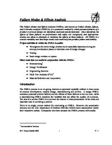
3.4. AN EXAMPLE FOR DEMONSTRATION In Section 2.3, an example was used to show the difference between a failure scenario and a failure mode, the same example is adopted here to demonstrate how the new method is applied to evaluate the risk of root cause. All of the failure scenarios initiated by a root cause are shown in Figure 2.2 in Section 2. Based upon the failure scenarios, a cause-effect chain structure is constructed as shown in Figure 3.2. In the structure, oil leak is the root cause CR , and the purpose of analysis is to find the total risk of CR in terms of expected cost. As seen from the structure, “Oil leak” as a root cause has two immediate effects, “Warning lights on” and “No warning lights”, and each of them serves as a cause in their own chains.

Signal detected

Operation ceased

Warning lights on

Signal undetected

Oil leak

No warning lights

Operation continues

Operation continues

Engine malfunction

Engine malfunction

Figure 3.2. An Example of Cause-Effect Chain Structures [27]

43

44

If warning lights turn on, and the signal is detected, then the end effect will be “Operation ceased”, and this means that the driver will send the car to be examined. On the other hand, if the signal is not detected, the driver will continue driving without noticing the oil leak, and this leads to the end effect “Engine malfunction”. Besides these two failure scenarios, there is another possibility that warning lights never turn on after oil leak. If this happens, the driver will also continue driving without noticing oil leak in the engine, and so the end effect in this failure scenario is “Engine malfunction” too. The simplified structure after substituting symbols into Figure 3.2 is shown below in Figure 3.3.

Figure 3.3. Simplified Structure after Substituting Symbols into Figure 3.2

45

In this case, for a root cause “Oil leak”, there exist three failure scenarios, in another word, three chains. To evaluate the risk, the risk of root cause in each chain should be analyzed separately first. Then add all the risk together in order to acquire the total risk of root cause for the whole structure. So the next step after the construction of such a structure will be collecting as much useful information from historical data as possible. Once the information about the occurrence probability of each element in the structure above and failure cost are both acquired, the risk of “Oil leak” in terms of cost can be calculated. The equations used to calculate the risks are displayed below. For path 1: CR  E11  D11  E12

R1 (CR )  P(CR ) P( E11 CR ) P( D11 ) P( E12 CR , E11, D11 )C1

(14)

For path 2: CR  E11  D11  E12  E13 R2 (CR )  P(CR ) P( E11 CR ) P( D11 ) P( E12 CR , E11 , D11 ) P( E13 CR , E11 , D11 , E12 ) C2

(15)

For path 3: CR  E21  E22  E23

R3 (CR )  P(CR ) P( E21 CR ) P( E22 CR , E21 ) P( E23 CR , E21, E22 ) C3

(16)

The total expected cost of root cause is given by

R(CR )  R1 (CR )  R2 (CR )  R3 (CR )

(17)

46

Now that all the equations used for calculating risks are obtained, the next step is collecting information on all of the elements in the equations, for example, the occurrence probability of root cause P(CR ) . The information is provided in Table 3.2 and Table 3.3. The values may change for other cases, since the information can vary significantly under different circumstances, for example, age of the car, regular maintenance history of the car, and so on.

Table 3.2. Probability Values

P(CR )

0.1

P( D11 )

0.95

P( D11 )

0.05

P( E11 CR )

0.97

P( E22 CR , E21 )

0.99

P( E21 CR )

0.03

P( E23 CR , E21 , E22 )

0.98

P( E12 CR , E11 , D11 )

P( E12 CR , E11 , D11 )

P( E13 CR , E11 , D11 , E12 )

0.99 0.94 0.99

Table 3.3. Failure Costs (in Dollars)

C1

500

C2

3000

C3

3000

47

With the information provided by Table 3.2 and Table 3.3, the risk of root cause for each path can be calculated as follows.

R1 (CR )  0.1 0.97  0.95  0.99  500  $45.61425

(18)

R2 (CR )  0.1 0.97  0.05  0.94  0.99  3000  $13.54023

(19)

R3 (CR )  0.1 0.03  0.99  0.98  3000  $8.7318

(20)

The total expected cost of root cause is then given by

R(CR )  45.61425  13.54023  8.7318  $67.88628

(21)

The total expected cost of root cause R(CR ) is about 68 dollars. In the next section, the new FMEA method will be applied to the turbine blades of the aforementioned hydrokinetic system. The expected costs of two root causes are evaluated and compared to each other so that the root cause with higher expected cost can be identified and corrective actions are taken to reduce the expected cost.

48

4. APPLICATION

In Section 3, a new FMEA approach was introduced. This approach uses the expected cost to evaluate the risk of root causes. In order to facilitate the process of risk analysis, a cause-effect chain structure which is based on failure scenarios is employed too. Failure scenarios can include all possible failures initiated by the same root cause, and this makes the result of the risk analysis more reliable and accurate. After constructing such a structure, information such as probabilities of root causes, conditional probabilities of intermediate effects and failure costs is collected from historical data and other sources. Then the risk of the root cause in terms of expected cost can be calculated easily. The objective of this research task is to evaluate and apply the new FMEA method to the hydrokinetic turbine design. The system is still under development, data are not sufficient. But we still conduct the application using historical data and other sources. Wind turbine and hydrokinetic turbine are quite similar to each other from both design and operation point of view, and thousands of wind turbines are in service right now, and data from wind turbines can serve as a source for the risk analysis on hydrokinetic turbines. However, the operation environment of hydrokinetic turbines is significantly different from that of wind turbines, and the data should be used selectively. At the meantime, data from hydrokinetic turbines that are deployed all over the world are collected as well when applying the new approach to the aforementioned hydrokinetic turbines.

49

In this section, details on how the new approach is applied to the hydrokinetic turbine system will be discussed. Since a turbine blade is the most critical component in the system, in this case study, we applied the new method to its design. Root causes and intermediate effects of turbine blades are examined to make sure all possible failure scenarios are considered.

4.1. FAILURE SCENARIOS OF TURBINE BLADES Root causes that might happen when the turbine is in operation are considered and all the possible failure scenarios that are initiated by the root causes are shown in Table 4.1. As can be observed from the first column in the table, there are in total six root causes. Each of them initiates a cause-effect chain structure. The second root cause, “Corrosive environment”, is used to demonstrate how to conduct the risk analysis. This root cause results in five different failure scenarios. Each scenario is analyzed separately, and then the results are aggregated together to obtain the total risk of this root cause.

4.2. CONSTRUCTING CAUSE-EFFECT CHAIN STRUCTURES As discussed in Section 3, such a structure is composed of several cause-effect chains which are connected at the beginning by the same root cause, and each chain represents a failure scenario that is initiated by the root cause.

Table 4.1. Failure Scenarios of Hydrokinetic Turbine Blades Tremendous change in flow velocity (0.1-0.2)

Overspeed rotation of blades (07-0.8)

Varying loads on blade (0.95)

E121 Local stress concentration (0.5-0.7)

CR Corrosive environment (0.6-0.8)

Impact on blades (0.01-0.02) Debris piling on blades (0.4-0.6) Impact on blades (0.7-0.8)

E122 Strength reduction (0.8-0.9)

D121 Undetected (0.01-0.05) D122 Detected (0.95-0.99) D122 Undetected (0.01-0.05)

System shutdown Fatigue(0.6-0.7)

E131 System shutdown

E131 Fatigue (0.6-0.7)

E141 Blade fracture (0.8-0.9)

E132 System shutdown

E132 Fatigue (0.6-0.7)

E123 Propagated cracks(0.4-0.5)

E133 Blade fracture(0.5-0.6)

Small deformation (0.5-0.1)

Reduced efficiency (0.5-0.7)

Increasing loads on system (0.5-0.7)

System shutdown (0.6-0.8)

Blade fracture (0.6-0.8)

Blade fracture (0.8-0.9)

E142 Blade fracture (0.8-0.9)

50

Presence of trivial debris (0.5-0.6) Presence of moderate debris (0.1-0.2) Presence of huge debris (0.01-0.02)

E11 Blade corrosion (0.65)

Detected (0.95-0.99) Undetected (0.01-0.05) D121 Detected (0.95-0.99)

51

Since one root cause corresponds to one cause-effect chain structure, so in order to construct as many structures as possible, we need to figure out all the possible root causes first. The cause-effect chain structure was constructed as shown in Figure 4.1.

Figure 4.1. A Cause-Effect Chain Structure of Hydrokinetic Turbine Blades

52

It is shown in the structure that root cause CR has only one immediate effect E11 , which is followed by three different subsequent effects E121 , E122 , and E123 . Then E121 goes under detection. D121 means successful detection of E121 so that end effect E131 happens. D121 means unsuccessful detection of E121 so that E131 happens, which is followed by an end effect E141 . Similarly, E122 goes under detection too and leads to two different end effects E132 and E142 . Since there is no detection technique for effect

E123 , the occurrence of E123 directly leads to end effect E133 . As mentioned before, all of the end effects will be evaluated in terms of cost, and so failure costs C1 , C2 , C3 , C4 and C5 are used to evaluate end effects E131 , E141 ,

E132 , E142 and E133 , respectively. Equation (22) through Equation (26) shown below calculate the risk of root cause for each chain. For path 1: CR  E11  E121  D121  E131 R1 (CR )  P(CR ) P( E11 CR ) P( E121 CR , E11 ) P( D121 ) P( E131 CR , E11 , E121 , D121 ) C1

(22)

For path 2: CR  E11  E121  D121  E131  E141 R2 (CR )  P(CR ) P( E11 CR ) P( E121 CR , E11 ) P( D121 ) P( E131 CR , E11 , E121 , D121 ) P( E141 CR , E11 , E121 , D121 , E131 )C2

(23)

53

For path 3: CR  E11  E122  D122  E132 R3 (CR )  P(CR ) P( E11 CR ) P( E122 CR , E11 ) P( D122 )

(24)

P( E132 CR , E11 , E122 , D122 ) C3

For path 4: CR  E11  E122  D122  E132  E142 R4 (CR )  P(CR ) P( E11 CR ) P( E122 CR , E11 ) P( D122 ) P( E132 CR , E11 , E122 , D122 )

(25)

P( E142 CR , E11 , E122 , D122 , E132 )C4

For path 5: CR  E11  E123  E133

R5 (CR )  P(CR ) P( E11 CR ) P( E123 CR , E11 ) P( E133 CR , E11, E123 ) C5

(26)

Equation (27) aggregates the results and acquires the total risk of root cause. The total expected cost of root cause is then given by

R(CR )  R1 (CR )  R2 (CR )  R3 (CR )  R4 (CR )  R5 (CR )

As can be observed from the equations, in order to obtain the total risk of root cause CR , information such as probabilities and failure costs should be collected.

(27)

54

4.3. COLLECTING INFORMATION ON THE HYDROKINETIC TURBINE Now the cause-effect chain structure is constructed, and how the risk is calculated is known as well. The next step is to collect information for each element in Equation (22) through Equation (26). 4.3.1. Probabilities of Failures. To obtain the probabilities of failures, information such as occurrence probabilities of root causes , conditional probabilities of intermediate effects, and probabilities of successful or unsuccessful detection should be estimated first. The probability values involved in the equations above are all shown in Table 4.2. As mentioned before, since information on hydrokinetic turbines is quite limited, historical data on wind turbines are adopted too, which will inevitably introduce more uncertainties to the probability values assigned to root causes and intermediate effects. So interval probabilities are employed here. For example, the occurrence probability of root cause “Tremendous change in flow rate and direction” which is the first cell in the first column of Table 4.1 is assigned to be “[0.1-0.2]”, because different rivers or streams have different current flow situations, even within the same river, the flow situation changes too. Interval probabilities can accommodate uncertainties due to insufficient data. When more data are available, these intervals can be modified to be more accurate so that the results are more accurate and reliable. Since some of the probabilities are in the form of intervals, it can be foreseen that expected costs will be in the form of intervals too. This means that the expected cost obtained by the new method can accommodate uncertainties too and allow for further modifications.

55

Table 4.2. Probability Values

P(CR )

0.6-0.8

P( D122 )

0.95-0.99

P( E11 CR )

0.65

P( D122 )

0.01-0.05

P( E121 CR , E11 )

0.5-0.7

P( E131 CR , E11 , E121 , D121 )

0.6-0.7

P( E122 CR , E11 )

0.8-0.9

P( E141 CR , E11 , E121 , D121 , E131 )

0.8-0.9

P( E123 CR , E11 )

0.4-0.5

P( E132 CR , E11 , E122 , D122 )

0.6-0.7

P( D121 )

0.95-0.99

P( E142 CR , E11 , E122 , D122 , E132 )

0.8-0.9

P( D121 )

0.01-0.05

P( E133 CR , E11 , E123 )

0.5-0.6

4.3.2. Costs of Failures. Once the probabilities of failures are available, the next step is to find the cost of failures. Time is a factor to determine the cost of failure. In order to obtain the cost of failures, detection time Tdt , fixing time T f and delay time Tdl should be acquired first. Detection time means the time to realize and identify a certain type of failure that has occurred and diagnose the exact location and its root cause. Fixing time is the time to fix each individual component. Delay time is the time incurred for on-value activities such as waiting for response from technicians. The unit for all the time information is in hours.

56

The failure cost mainly includes three components: labor cost Cl , material cost

Cm and opportunity cost Co . The meanings of labor cost and material cost are explicit by their names. The opportunity cost is the cost that incurs when a failure inhibits the main function of the system and prevents any value creation. The labor cost can be derived with the aforementioned time information using the following equation: Cl  (Tdt  Tf  Tdl )  Rl  N

(28)

where Rl means labor rate, and N represents the number of operators that are assigned to fix problems. The material cost can be obtained using the following equation: Cm  C p  N p

(29)

where C p means the cost of part, and N p represents the number of parts that need to be replaced. The opportunity cost is calculated using the following equation: Co  (Tdt  Tf  Tdl )  Ro

where Ro means hourly opportunity cost. The labor cost and opportunity cost are dependent on time and once the time information is obtained through historical data, they can be estimated easily.

(30)

57

After examining the cause-effect chain structure in Figure 4.1, we noticed that there are two different types of failures, “Blade fracture” and “System shutdown”. For the first failure, “Blade fracture”, the cost will be the summation of labor cost, material cost and opportunity cost. However, for the second failure, “System shutdown”, the cost will be the summation of labor cost and opportunity cost only, because in this case blades do not need to be replaced yet. And it can also be foreseen that the labor cost and opportunity cost involved in the second failure will be less than that involved in the first one, because the time of maintenance after system shutdown will be less than the time of replacing fractured blades. Table 4.3 shows the comparison of the time loss between the two different failures.

Table 4.3. Loss Time of the Two Failures (in Hours) Blades fracture

System shutdown

Detection time

5

1

Fixing time

4

2

Delay time

4

2

Total time

13

5

58

The labor rate in this analysis is assumed to be $50 per hour. Suppose two operators are assigned to fix problems after either of the two failures happens. The labor cost for either of the two failures can be calculated with Equation (28). From Equation (29) it can be seen that the material cost is independent of time, and it is only related to the cost of parts to be replaced and the quantity of the parts. Since this case study is focused upon turbine blades of the hydrokinetic system, the two failures are only related to turbine blades too. The manufacturing cost of the turbine blades is about $2500. The hourly opportunity cost is composed of the labor rate as well as the loss of electrical power that is generated from the hydrokinetic system per hour, considering the system will be shut down when failure happens. The turbine blades used for this case study are very small in size, and the length of blade is about 0.3 m. The power generated by the system is relatively small, and so the failure-resulted loss of electric power may be neglected. After conducting sufficient research on other turbines that have been deployed, it is estimated that the hourly opportunity cost for this hydrokinetic system is about $500, which is relatively low because of the small size of the system. According to Equation (30), the opportunity cost when either of two failures happens can then be calculated. The comparison of the costs between the two different failures is shown in Table 4.4.

59

Table 4.4. Costs of the Two Failures (in Dollars) Blade fracture

System shutdown

Labor cost

1300

500

Material cost

2500

100

Opportunity cost

6500

2500

Total cost

10300

3100

It should be pointed out that the hydrokinetic system in this case study is much smaller compared to those tested in reality, so the failure costs for this system can be significantly magnified when the system is scaled up. For example, if the blades are lengthened and widened, the material cost will be higher when failure happens. The opportunity cost will be higher too because the shutdown of a larger system means increased loss of electrical power that should have been generated.

4.4. CALCULATING RISK IN TERMS OF EXPECTED COST Now that the probability values are obtained and shown in Table 4.2, and the failure costs are listed in Table 4.4. Plugging the values in the two tables into Equation (22) through Equation (26) will yield the risk of root cause for each path. Then Equation (27) adds all the risks together and yields the total risk of root cause

R(CR ) .

60

As mentioned before, since some of the probability values are intervals, the total risk, which is in terms of expected cost, will be an interval too. So the lower bound and upper bound need be found, separately. The lower bound for each path is calculated by the following Equation (31) through Equation (35).

R1 (CR )l  0.6  0.65  0.5  0.95  3100  $547.275

(31)

R2 (CR )l  0.6  0.5  0.6  0.01 0.6  0.8 10300  $8.8992

(32)

R3 (CR )l  0.6  0.65  0.8  0.95  3100  $918.84

(33)

R4 (CR )l  0.6  0.65  0.8  0.01 0.6  0.8 10300  $15.42528

(34)

R5 (CR )l  0.6  0.65  0.4  0.5  3100  $241.8

(35)

The lower bound of the total expected cost of root cause is given by

R(CR )l  R1 (CR )l  R2 (CR )l  R3 (CR )l  R4 (CR )l  R5 (CR )l  547.275  8.8992  918.84  15.42528  241.8

(36)

 $1732.23948

The upper bound for each path is calculated by the following Equation (37) through Equation (41).

R1 (CR )u  0.8  0.65  0.7  0.99  3100  $1117.116

(37)

R2 (CR )u  0.8  0.65  0.7  0.05  0.7  0.9 10300  $118.0998

(38)

61

R3 (CR )u  0.8  0.65  0.9  0.99  3100  $1436.292

(39)

R4 (CR )u  0.8  0.65  0.9  0.05  0.7  0.9 10300  $151.8426

(40)

R5 (CR )u  0.8  0.65  0.5  0.6  3100  $483.6

(41)

The upper bound of the total expected cost of root cause is given by

R(CR )u  R1 (CR )u  R2 (CR )u  R3 (CR )u  R4 (CR )u  R5 (CR )u  1117.116  118.0998  1436.292  151.8426  483.6

(42)

 $3306.9504

The expected cost of root cause R(CR ) is given by

$1732  R(CR )  $3307

(43)

4.5. ANOTHER CASE STUDY For the purpose of comparing risks of different root causes, the first root cause in Table 4.1, “Tremendous change in flow velocity and direction” was used to conduct another case study. The cause-effect chain structure is shown in Figure 4.2. The risk of CR in each path is calculated by the following equations. For path 1: CR  E11  E12  D12  E13 R1 (CR )  P(CR ) P( E11 CR ) P( E12 CR , E11 ) P( D12 ) P( E13 CR , E11 , E12 , D12 )C1

For path 2: CR  E11  E12  D12  E13  E14

(44)

62

R2 (CR )  P(CR ) P( E11 CR ) P( E12 CR , E11 ) P( D12 ) P( E13 CR , E11 , E12 , D12 ) (45)

P( E14 CR , E11 , E12 D12 , E13 )C2

Figure 4.2. Another Cause-Effect Chain Structure of Hydrokinetic Turbine Blades

Next, information is collected and shown in Table 4.5 and Table 4.6 below.

Table 4.5. Probability Values P( D12 )

P(CR )

0.1-0.2

P( E11 CR )

0.7-0.8

P( E12 CR , E11 )

0.95

P( D12 )

0.95-0.99

P( E13 CR , E11 , E12 , D12 ) P( E14 CR , E11 , E12 D12 , E13 )

0.01-0.05 0.6-0.7 0.8-0.9

63

Table 4.6. Loss Time of the Two Failures (in Hours) System shutdown Blade fracture Detection time

3

5

Fixing time

2

4

Delay time

4

4

Total time

9

13

As discussed in Section 4.4, the labor rate is estimated to be $50 per hour, the hourly opportunity cost is about $500, and the material cost for the turbine blades is $2500. With Equations (23), (24) and (25), and Table 4.6, the costs of the two failures are calculated and shown in Table 4.7.

Table 4.7. Costs of the Two Failures (in Dollars) System shutdown Blade fracture Labor cost

900

1300

Material cost

200

2500

Opportunity cost

4500

6500

Total failure cost

5600

10300

64

The probability values are shown in Table 4.5 and the failure costs are shown in Table 4.7. Plugging these values into Equation (44) and (45) yields the risk of root cause for each path. Since only the two paths are initiated by root cause CR , the risk of CR is obtained by adding the results of Equation (44) and Equation (45) together.

R(CR )  R1 (CR )  R2 (CR )

(46)

The lower bound of the expected cost for each path is calculated by Equation (47) and Equation (48).

R1 (CR )l  0.1 0.7  0.95  0.95  5600  $353.78

(47)

R2 (CR )l  0.1 0.7  0.95  0.01 0.6  0.8 10300  $32.8776

(48)

The lower bound of the total expected cost of root cause is given by

R(CR )l  R1 (CR )l  R2 (CR )l  353.78  32.8776  $386.6576

(49)

The upper bound of the expected cost for each path is calculated by Equation (50) and Equation (51).

R1 (CR )u  0.2  0.8  0.95  0.99  5600  $842.688

(50)

R2 (CR )u  0.2  0.8  0.95  0.05  0.7  0.9 10300  $49.3164

(51)

The upper bound of the total expected cost of root cause is given by

65

R(CR )u  R1 (CR )u  R2 (CR )u  842.688  49.3164  $892.0044

(52)

The total expected cost of the root cause R(CR ) is given by

$387  R(CR )  $892

(53)

4.6. COMPARISON OF RISKS BETWEEN TWO CASE STUDIES The comparison of interval risks between the two root causes are shown in Table 4.8.

Table 4.8. Comparison of Interval Risks (in Dollars)

CR

R(CR )l

R(CR )u

Corrosive environment

1732

3307

Tremendous change in flow velocity

387

892

It is quite obvious that the first root cause has higher risk, because both the lower bound and upper bound of the first root cause are higher than those of the second one. And the two ranges have no intersection in between, which makes the comparison straightforward. The first root cause “Corrosive environment” has higher risk and corrective actions should be taken with priority to reduce the risk.

66

However, for other cases, when risks are compared with each other, it is very likely that an intersection exists between two risk intervals. If this happens, comparison is not straightforward anymore. Different approaches on decision making under interval probabilities have been made. The approaches can be found in [48-51]. However, in this paper, two general approaches are proposed to address this issue. One is to directly compare the average value of the two intervals. The other one is the worst case approach, which only compares the upper bound of the two intervals.

67

5. CONCLUSIONS AND FUTURE WORK

In the traditional FMEA method, risk is evaluated by risk priority number (RPN), which is the product of O (occurrence), S (severity), and D (detection). Failure modes with higher RPN values are considered having higher risks. Corrective actions are then taken to reduce the RPN values. This method has been implemented in industry since last century. However, it has the following drawbacks: 

The subjectivity in RPNs is considerably high.



The comparison of RPNs between products or processes is difficult.



The accuracy and reliability of the results provided by the traditional FMEA are questionable. Many methods have been developed for improving FMEA. The methodology

proposed in this work employs the expected cost as the tool to evaluate risks so that the subjectivity in risk results can be minimized and comparison of risks is facilitated. Moreover, the new method uses the cause-effect chain structure to represent failure scenarios given a root cause so that more possible end effects are under consideration, and the results become more accurate and reliable.

5.1. CONCLUSIONS In this work, a modified FMEA approach is proposed and demonstrated. It is applied to the hydrokinetic system being developed at Missouri S&T to evaluate the risks of root causes that might incur failures to turbine blades of the system. This new approach proved its advantages over the traditional way in the following aspects:

68



First, the new method employs cause-effect chain structures which are constructed based upon failure scenarios and the Bayesian network. The structures overcome the following drawback of the traditional FMEA: only the most serious end effects are taken into account to calculate the RPN. However, this is not the case in reality, because several different end effects are all possible to occur even if there is only one root cause. The implementation of failure scenarios and Bayesian network can take many possible end effects into consideration, and in a cause-effect chain structure, all possibilities from a root cause are included. This makes the results of risk analysis more accurate and reliable.



Second, RPN as the key element in the traditional FMEA method has always been most criticized. When conducting FMEA, assigning precise ratings for O (occurrence), S (severity), and D (detection) is difficult, especially when historical data are not available. The RPNs are considered subjective because sometimes the experience of the team members is the only source of information. However, the new method does not employ RPN as the tool to evaluate risk; instead, occurrence and severity ratings are substituted by the expected cost, which is adopted as a new tool to evaluate risks. In this way, not only more reasonable results can be obtained, but also the subjectivity of the results can be reduced.



Moreover, in the new method, the detection rating is replaced by the probability of either successful or unsuccessful detection, which is directly related to the maturity of detection techniques implemented in applications. This makes the results more reliable and realistic.

69



Last, in the traditional FMEA, comparison of risk information represented by RPNs is quite difficult and sometimes impossible. In this new method, risk is evaluated by expected cost, which makes the comparison of risk information straightforward.

5.2. FUTURE WORK Although the new method improves the traditional FMEA, there is room for further improvement. In the method proposed in this paper, risk is evaluated in terms of expected cost, which is the product of the probability of failure and failure cost. Since the information on probabilities and costs are all obtained from historical data and sometimes appropriate assumptions, uncertainties exist in the components of expected cost, such as detection time, fixing time and so on. Sensitive analysis can be conducted on these components to determine which of them has the most significant influence on the risk results. Then the accuracy and reliability of the results can be improved efficiently by reducing uncertainty in this component. Hydrokinetic technologies are still in the developmental phase, and not many turbines have been built and deployed for commercial use, so data for hydrokinetic turbines are very limited by far. In the application of the proposed method to the hydrokinetic turbine, interval probabilities are used to accommodate uncertainties due to insufficient data. However, the intervals can be modified to represent the real situation more precisely when more hydrokinetic systems are deployed in rivers or oceans. Risks with higher accuracy and reliability can be obtained.

70

Moreover, when comparing the two interval risks in Section 4, it involves the technique of decision making under interval probabilities. Although two approaches are made to address this issue, a more reliable method needs to be conceived.

71

BIBLIOGRAPHY

[1].

SAE. "Design Analysis Procedure For Failure Modes, Effects and Criticality Analysis (FMECA)." SAE International, 1967.

[2].

Matsumoto, K., Matsumoto, T., and Goto, Y. "Reliability Analysis of Catalytic Converter as an Automotive Emission Control System," SAE Prepr, No. 750178, 1975.

[3].

Tague, N. R. The Quality Toolbox: Asq Press, 2005.

[4].

Arvanitoyannis, I. S., and Varzakas, T. H. "Application of ISO 22000 and Failure Mode and Effect Analysis (FMEA) for industrial processing of salmon: A case study," Critical Reviews in Food Science and Nutrition Vol. 48, No. 5, 2008, pp. 411-429.

[5].

Scipioni, A., Saccarola, G., Centazzo, A., and Arena, F. "FMEA methodology design, implementation and integration with HACCP system in a food company," Food Control Vol. 13, No. 8, 2002, pp. 495-501.

[6].

Liu, H.-T. "The extension of fuzzy QFD: From product planning to part deployment," Expert Systems with Applications Vol. 36, No. 8, 2009, pp. 1113111144.

[7].

Chen, L. H., and Ko, W. C. "Fuzzy linear programming models for new product design using QFD with FMEA," Applied Mathematical Modelling Vol. 33, No. 2, 2009, pp. 633-647.

[8].

Bowles, J. B., and Peláez, C. E. "Fuzzy logic prioritization of failures in a system failure mode, effects and criticality analysis," Reliability Engineering and System Safety Vol. 50, No. 2, 1995, pp. 203-213.

[9].

Pillay, A., and Wang, J. "Modified failure mode and effects analysis using approximate reasoning," Reliability Engineering and System Safety Vol. 79, No. 1, 2003, pp. 69-85.

72

[10].

Duminică, D., and Avram, M. "Criticality Assessment Using Fuzzy Risk Priority Numbers."

[11].

Gargama, H., and Chaturvedi, S. K. "Criticality assessment models for failure mode effects and criticality analysis using fuzzy logic," IEEE Transactions on Reliability Vol. 60, No. 1, 2011, pp. 102-110.

[12].

Gan, L., Pang, Y., Liao, Q., Xiao, N. C., and Huang, H. Z. "Fuzzy criticality assessment of FMECA for the SADA based on modified FWGM algorithm & centroid deffuzzification." 2011, pp. 195-202.

[13].

Guimarães, A. C. F., and Lapa, C. M. F. "Fuzzy FMEA applied to PWR chemical and volume control system," Progress in Nuclear Energy Vol. 44, No. 3, 2004, pp. 191-213.

[14].

Guimarães, A. C. F., and Lapa, C. M. F. "Fuzzy inference to risk assessment on nuclear engineering systems," Applied Soft Computing Journal Vol. 7, No. 1, 2007, pp. 17-28.

[15].

Zafiropoulos, E. P., and Dialynas, E. N. "Reliability prediction and failure mode effects and criticality analysis (FMECA) of electronic devices using fuzzy logic," International Journal of Quality and Reliability Management Vol. 22, No. 2, 2005, pp. 183-200.

[16].

Sharma, R. K., Kumar, D., and Kumar, P. "Systematic failure mode effect analysis (FMEA) using fuzzy linguistic modelling," International Journal of Quality and Reliability Management Vol. 22, No. 9, 2005, pp. 986-1004.

[17].

Bevilacqua, M., Braglia, M., and Gabbrielli, R. "Monte Carlo simulation approach for a modified FMECA in a power plant," Quality and Reliability Engineering International Vol. 16, No. 4, 2000, pp. 313-324.

[18].

Von Ahsen, A. "Cost-oriented failure mode and effects analysis," International Journal of Quality and Reliability Management Vol. 25, No. 5, 2008, pp. 466-476.

73

[19].

Seo, K. K., Park, J. H., Jang, D. S., and Wallace, D. "Approximate estimation of the product life cycle cost using artificial neural networks in conceptual design," International Journal of Advanced Manufacturing Technology Vol. 19, No. 6, 2002, pp. 461-471.

[20].

Jiang, Z. H., Shu, L. H., and Benhabib, B. "Reliability analysis of non-constantsize part populations in design for remanufacture," Journal of Mechanical Design, Transactions of the ASME Vol. 122, No. 2, 2000, pp. 172-178.

[21].

Roser, C., Kazmer, D., and Rinderle, J. "An economic design change method," Journal of Mechanical Design, Transactions of the ASME Vol. 125, No. 2, 2003, pp. 233-239.

[22].

Lee, B. H. "Using Bayes belief networks in industrial FMEA modeling and analysis." 2001, pp. 7-15.

[23].

He, D., and Adamyan, A. "An impact analysis methodology for design of products and processes for reliability and quality." Vol. 3, 2001, pp. 209-217.

[24].

Gilchrist, W. "Modelling Failure Modes and Effects Analysis," International Journal of Quality & Reliability Management Vol. 10, No. 5, 1993, pp. 16-23.

[25].

Rhee, S. J., and Ishii, K. "Life cost-based FMEA incorporating data uncertainty." Vol. 3, 2002, pp. 309-318.

[26].

Rhee, S. J., and Ishii, K. "Life Cost-Based FMEA Using Empirical Data." Vol. 3, 2003, pp. 167-175.

[27].

Kmenta, S., and Ishii, K. "Scenario-based FMEA: a life cycle cost perspective," Proc. ASME Design Engineering Technical Conf. Baltimore, MD. 2000.

[28].

Kmenta, S., and Ishii, K. "Scenario-based failure modes and effects analysis using expected cost," Journal of Mechanical Design, Transactions of the ASME Vol. 126, No. 6, 2004, pp. 1027-1035.

74

[29].

Stamatis, D. H. Failure Mode and Effect Analysis: Fmea from Theory to Execution: American Society for Quality, 2003.

[30].

Sankar, N. R., and Prabhu, B. S. "Modified approach for prioritization of failures in a system failure mode and effects analysis," International Journal of Quality & Reliability Management Vol. 18, No. 3, 2000, pp. 324-335.

[31].

B.S., N. "Solutions for the Improvement of the Failure Mode and Effects Analysis in the Automotive Industry," Recent Researches in Manufacturing Engineering, pp. 127-132.

[32].

Rhee, S. J., and Ishii, K. "Using cost based FMEA to enhance reliability and serviceability," Advanced Engineering Informatics Vol. 17, No. 3-4, 2003, pp. 179-188.

[33].

Anleitner, M. A. The Power of Deduction: Failure Modes and Effects Analysis for Design: ASQ Quality Press, 2010.

[34].

Kusakana, K., and Vermaak, H. J. "Hydrokinetic power generation for rural electricity supply: Case of South Africa," Renewable Energy Vol. 55, 2013, pp. 467-473.

[35].

Pusapati, G. "Transmission Shaft Design for Hydrokinetic Turbine with Reliability Consideration," Mechanical Engineering. Vol. Master of Science, Missouri University of Science and Technology, 2013.

[36].

Date, A., and Akbarzadeh, A. "Design and cost analysis of low head simple reaction hydro turbine for remote area power supply," Renewable Energy Vol. 34, No. 2, 2009, pp. 409-415.

[37].

Güney, M. S., and Kaygusuz, K. "Hydrokinetic energy conversion systems: A technology status review," Renewable and Sustainable Energy Reviews Vol. 14, No. 9, 2010, pp. 2996-3004.

75

[38]. Hall, D. G., Reeves, K. S., Brizzee, J., Lee, R. D., Carroll, G. R., and Sommers, G. L. "Feasibility Assessment of the Water Energy Resources of the United States for New Low Power and Small Hydro Classes of Hydroelectric Plants." IDAHO National Laboratory, 2006.

[39].

Hall, D. G., Cherry, S. J., Reeves, K. S., Lee, R. D., Carroll, G. R., Sommers, G. L., and Verdin, K. L. "Water Energy Resources of the United States with Emphasis on Low Head/Low Power Resources." IDAHO National Engineering and Environmental Laboratory, 2004.

[40].

Khan, M. J., Iqbal, M. T., and Quaicoe, J. E. "River current energy conversion systems: Progress, prospects and challenges," Renewable and Sustainable Energy Reviews Vol. 12, No. 8, 2008, pp. 2177-2193.

[41].

Khan, M. J., Bhuyan, G., Iqbal, M. T., and Quaicoe, J. E. "Hydrokinetic energy conversion systems and assessment of horizontal and vertical axis turbines for river and tidal applications: A technology status review," Applied Energy Vol. 86, No. 10, 2009, pp. 1823-1835.

[42].

Bedard, R. "Prioritized Research, Development, Deployment and Demonstration Needs: Marine and Other Hydrokinetic Renewable Energy ". Electric Power Research Institute, 2008.

[43].

"International Energy Outlook 2011, World energy demand and economic outlook."

[44].

Arabian-Hoseynabadi, H., Oraee, H., and Tavner, P. J. "Failure Modes and Effects Analysis (FMEA) for wind turbines," International Journal of Electrical Power and Energy Systems Vol. 32, No. 7, 2010, pp. 817-824.

[45].

Kahrobaee, S., and Asgarpoor, S. "Risk-based failure mode and effect analysis for wind turbines (RB-FMEA)." 2011.

[46].

Heckman, A., Rovey, J. L., Chandrashekhara, K., Watkins, S. E., Mishra, R., and Stutts, D. "Ultrasonic underwater transmission of composite turbine blade structural health." Vol. 8343, 2012.

76

[47].

Mock, T. J., and Grove, H. D. Measurement, accounting, and organizational information: John Wiley & Sons Australia, Limited, 1979.

[48].

Guo, P., and Tanaka, H. "Decision making with interval probabilities," European Journal of Operational Research Vol. 203, No. 2, 2010, pp. 444-454.

[49].

Engemann, K. J., and Yager, R. R. "A general approach to decision making with interval probabilities," International Journal of General Systems Vol. 30, No. 6, 2001, pp. 623-647.

[50].

He, D. Y., and Zhou, R. X. "On methods of decision-making under interval probabilities." 2009, pp. 277-282.

[51].

Liu, L., Chen, Y. X., and Ge, Z. H. "Probability measure of interval-number based on normal distribution and multi-attribute decision making," Xi Tong Gong Cheng Yu Dian Zi Ji Shu/Systems Engineering and Electronics Vol. 30, No. 4, 2008, pp. 652-654.

77

VITA

Liang Xie was born on August 13th, 1987 in a town in Hubei province, China. He got his Bachelor of Engineering degree at Huazhong Agricultural University in 2009. Then after one and half years of preparation, he came to the United States in 2011 to pursue his Master’s degree. And he got his Master of Science degree under supervision of Dr. Xiaoping Du at Missouri University of Science and Technology in August 2013.