A MULTI-SPECIES BIO-ECONOMIC MODEL FOR INTEGRATED WEED MANAGEMENT
Marta Monjardino, David Pannell and Stephen Powles
Paper presented at the 45th Annual Conference of the Australian Agricultural and Resource Economics Society, January 23 to 25, 2001, Adelaide, South Australia.
Copyright 2001 by Marta Monjardino, David Pannell and Stephen Powles. All rights reserved. Readers may make verbatim copies of this document for non-commercial purposes by any means, provided that this copyright notice appears on all such copies.
A MULTI-SPECIES BIO-ECONOMIC MODEL FOR INTEGRATED WEED MANAGEMENT Marta Monjardino1,2, David Pannell1 and Stephen Powles2 1
Agricultural and Resource Economics Western Australian Herbicide Resistance Initiative University of Western Australia, 35 Stirling Hwy, Crawley WA 6009 2
ABSTRACT A multi-species version of the bio-economic RIM (Resistance and Integrated Management) model has been developed to deal with the complexities involved in the long-term integrated management of annual ryegrass (Lolium rigidum Gaud.) and wild radish (Raphanus raphanistrum L.), which dominate and co-exist in southern Australia. In this paper, we present a review of the existing options on how to model multi-species competition in order to select the best approach for incorporation in the RIM framework. Furthermore, we show how we have extended the original single-species ryegrass RIM model to include other aspects of the wild radish biology as well as a set of extra weed management practices used to control this weed species. We also demonstrate how the Multi-species RIM model can be used to evaluate weed management scenarios of co-existing herbicide resistant species. This is done through investigating the implications of using Roundup Ready® canola in the system. Key words: bio-economics, multi-species model, ryegrass, wild radish, herbicide resistance, integrated weed management, herbicide-tolerant crops, Roundup Ready® canola
INTRODUCTION Weed infestations in agriculture usually consist of a number of co-existing weed species. Hence, interactions between weeds and crops and within weeds should be considered in studies of crop yield loss and in strategies for weed management (Poole and Gill, 1987; Combellack and Friesen, 1992). However, experiments with multiple species can be large and complex, with their thorough analyses requiring the development of appropriate mathematical tools (Ball and Shaffer, 1993; Van Acker, Lutman and Froud-Williams, 1998). Improved modelling capabilities of multi-species interactions are therefore important to the full understanding and management of current agricultural systems. In southern Australia, annual ryegrass (Lolium rigidum Gaud.) and wild radish (Raphanus raphanistrum L.) frequently co-exist and are economically very important. Recent field surveys conducted throughout the wheatbelt of Western Australia indicated that about 70 and 20 percent of the surveyed ryegrass and wild radish populations showed some level of herbicide resistance, respectively (Llewellyn and Powles, 2001; Walsh, Duane and Powles, 2001). The situation is now such that farmers no longer can rely solely on herbicides for effective weed control, but rather need to combine a range of chemical and non-chemical methods (IWM) to control these species. Hence, a multi-species version of the bio-economic RIM model has been developed to deal with the complexities involved in the simultaneous integrated management of annual ryegrass and wild radish over time.
2
In this paper, we present a review of the existing options on how to model multi-species competition in order to select the best approach for incorporation in the RIM framework. Furthermore, we show how we have extended the single-species ryegrass RIM model to include other aspects of the wild radish biology as well as a set of extra weed management practices used to control this weed species. Finally, we demonstrate how the multi-species RIM model can be used to evaluate the economic trade-offs between short-term costs and long-term benefits associated with the integrated management of co-existing herbicide resistant annual ryegrass and wild radish. This is done through investigating the implications of using Roundup Ready® canola in a realistic situation, which considers crucial biological and management interactions of two different weeds infesting the same farming system.
MODELLING MULTI-SPECIES COMPETITION A few models relating crop yield to the presence of more than one weed have been proposed in the literature (De Wit, 1960; Firbank and Watkinson, 1985; Street et al., 1985; Halse, 1986; Blackshaw, 1986; Hume, 1989 and 1993; Kropff and Spitters, 1991; Wilkerson, Modena and Coble, 1991; Kiniry et al., 1992; Ball and Shaffer, 1993; Swinton et al., 1994; Pannell and Gill, 1994; Trenbath and Stern, 1995; Sattin, Berti and Zanin, 1996). The performance of these models is summarized in Table 1 and evaluated according to the criteria presented below. Evaluation criteria The selection of a particular multi-species competition approach for use in this study was based on the following criteria for the indicated reasons: 1. A single-function approach, not a short-time-step dynamic simulation model. This decision is based on the fact that a single function is more convenient, faster to solve and more compatible with the general approach in the existing RIM model. Biological simulation models are thus excluded from the current selection process. 2. The function should be based on plant densities rather then on leaf area indices (LAIs). Density may often not be as accurate a measure of weed quantities in a field, as it does not account for patchiness, size of the weed and emergence flushes of the weeds (Parker and Murdoch, 1996). However, advantages of the density approach are that it relies on more readily available data, allowing for validity checking, is more practical for extra data collection and, is more compatible with the existing RIM model framework than the LAI approach. 3. A function capable of capturing the realistic features of crop-weed competition. In particular, if crop yield is a function of the weed density, Y = f(W), then the function should have the following characteristics: a) dY/dW < 0, for all W b) d2Y/dW2 > 0, for all W c) f(0) = max (Y) = 1, if expressed as a proportion of maximum yield. d) Has potential to be parameterized in such a way that f()> 0
3 4. Effects of a weed on crop yield may depend on the density of another weed, i.e. weed effects interact (De Wit, 1960; Alex, 1970; Kroh and Stephenson, 1980; Pannell and Gill, 1994). 5. A function capable of representing different crop plant densities. The reason for this is that high crop density is a strategy being recommended to farmers, which may as well be part of the optimal management strategy in the RIM model. 6. High densities of different weeds result in different minimum crop yields (Pannell and Gill, 1994). Previous approaches to multi-species competition The existing models or functions that deal with multi-species competition are listed in Table 1, following chronological order of their original publication. The performance of each model is further evaluated in terms of the selected criteria defined above. For convenience, the review is limited to models based on a single function, excluding the dynamic simulation models ALMANAC (Kiniry et al., 1992) and NTRM-MSC (Nitrogen, Tillage, Residue, Management- Multiple Species Competition) (Ball and Shaffer, 1993).
Table 1. Existing multi-species competition models according to the evaluation criteria. Multi-species functions 1 Single function A) De Wit, 1960 B) Firbank & Watkinson, 1985 C) Street et al., 1985 D) Blackshaw, 1986 E) Halse, 1986 F) Hume, 1989 & 1993 G) Kropff & Spitters, 1991 H) Wilkerson et al., 1991 I) Swinton et al., 1994 J) Pannell & Gill, 1994 K) Trenbath & Stern, 1995 L) Sattin et al., 1996
2 Densitybased function
Evaluation criteria 3 4 Weed All features effects /weed-crop interact competition
5 Different crop densities
6 Different minimum yields
Preferred multi-species approach When weighing up all the criteria in order to select the best multi-species approach to include in RIM, four of the presented models fail only one criterion: Model A Model B Model E Model J
4 It is judged that criterion 6 is less important than criterion 5, since meeting criterion 5 is essential to represent a weed management strategy that is being widely advocated (increasing crop seeding rates). Therefore, approach J is not used. Model A is also rejected, because it imposes unrealistic restrictions on the function (total yield is constant regardless of the combination of plant densities). In choosing between the other two, which are actually rather similar, model B is preferred because it is convenient to base parameter values on the existing single-weed version of RIM, which uses a function similar to model B. The preferred approach (B), estimates the effect of weed-crop competition on the production of crop grain/weed seed by using an adapted version of the model proposed by Firbank and Watkinson (1985). The single-weed version of the original function was modified by Maxwell, Roush and Radosevich. (1990) and by Diggle, Gill and Holmes. (1994) to become: Y
m P1 a P1 (k 2.1 P 2)
(1)
Where, Y = Yield or seed produced per plant m = Maximum seed production from the plants of species 1 in the absence of competition P1 = Density of the producing plant species (e.g. crop) P2 = Density of the competing plant species (e.g. weed) a= Constant for the crop being considered k2.1 = Competition effect of species 2 on species 1
This function has the potential to be modified in order to accommodate more species. This is done in a way similar to Halse’s model (E) by adding (kn.1 Pn) to the denominator of the equation, as illustrated in the next section.
THE MULTI-SPECIES RIM MODEL The Multi-species RIM (Resistance and Integrated Management) is a bio-economic model that simulates the population dynamics of annual ryegrass and wild radish over a 20-year period It is a decision support tool designed specifically for the evaluation of various management strategies to control herbicide-resistant weeds in dryland agriculture. The model includes a detailed representation of the biology of weeds, crops and pasture as well as of the economics of agricultural production and management. The outputs of the model are weed seed bank/density and profit, as illustrated by the RIM flow-chart (Figure 1). In this section, we give an overview of the model and show how the original ryegrass single-species RIM model (Pannell et al., 1999a). has been modified to include a second weed species, wild radish.
5
Figure 1. RIM flow-chart.
Weed biology Population dynamics The growth and mortality of ryegrass and wild radish weeds are represented in RIM according to the following equation based on Gorddard, Pannell and Hertzler (1996).
W V G (1 Ms ) (1 Mn ) (1 Mc)
(2)
Where, W = Density of weeds which survive to maturity V = Viable seeds present at the beginning of a given year G = Proportion of initial seed pool that germinates Ms = Proportion of germinated seeds that die naturally over summer Mn = Proportion of germinated seeds that are killed by non-chemical control Mc = Proportion of germinated seeds that are killed by herbicide application
Seeds that remain dormant, and hence do not germinate (1-G), either die naturally or add to the following year’s seed bank. The number of seeds present at the start of each season results thus from the amount of seed produced in spring plus the viable seed carried over form the previous year. Figure 2 illustrates the germination pattern of ryegrass and wild radish, based on the values shown in Table 2. Despite evidence that some wild radish seeds go through cycles of increased and decreased dormancy during the growing season (secondary dormancy, possibly caused by a drop in temperature at the start of that period) (Cheam, 1986), not enough information was available to allow for quantification of this phenomenon in the model.
% Germination of total initial seed bank
6
50 40 30
Ryegrass Wild radish
20 10 0 In-crop
1Season 2 10 days 3 2020days 5 days4 herbicides break
Time
Figure 2. Germination pattern of ryegrass and wild radish (adapted from Cheam, 1986 and Pannell et al., 1999a).
Table 2 summarises the model default key factors (adjustable by the user), which drive the pattern of weed population change over time. Next to weed seed germination by cohort relative to the crop, the model accounts for natural mortality of seeds and seedlings. The latter is assumed to be density-dependant at high seedling densities (2 percent mortality above 5000 ryegrass and 500 wild radish seedlings per m2). The effect of weed-crop competition on seed production and the impact of control practices to reduce weeds or seeds are dealt with in other sections of this paper.
Table 2. RIM parameters associated with population dynamics of ryegrass and wild radish. Biological variables Total % germination % Germination of cohort 1 (prior to 1st chance to seed)* % Germination of cohort 2 (1-10 days after break)* % Germination of cohort 3 (11-20 days after break)* % Germination of cohort 4 (before in-crop herbicides)* % Germination of cohort 5 (after in-crop herbicides)* Natural mortality of seedlings (% of total seedlings) Natural mortality of dormant seeds during season Natural mortality of seeds over summer
Ryegrass 82% 5% 38% 23% 14% 2% 2% 20% 30%
Wild radish 30% 4% 12% 8% 5% 1% 2% 5% 10%
* Germination here refers to % of total initial seed bank, whereas in the RIM model these figures are scaled to give the % germination of seeds remaining in the seed bank.
Seed production The preferred approach represented in (Equation 1) has been modified further to predict weed seed production in a multi-species situation (Equation 3) The multi-species equation includes
7 features of Halse’s model (E) such as a function of total plant density and the way the third species is included. Y PT
m P1 a P1 (k 2.1 P 2) (k 3.1 P 3)
(3)
Where, Y = Seed produced per plant for a particular weed species PT = A function of total plant density, which normally equals 1 m = Maximum seed production from the plants of species 1 in the absence of competition (Equation 4) P1 = Density of the producing plant species (e.g. the weed for which we are predicting seed production) P2 = Density of the first competing plant species (e.g. second weed species) P3 = Density of the second competing plant species (e.g. crop) a= Constant for the species being considered k2.1 = Competition effect of species 2 on species 1 k3.1 = Competition effect of species 3 on species 1
The maximum seed production (m) from the producing species in the absence of competition, was proposed by Diggle, Gill and Holmes (1994) to be given by the following equation: m
( M 0 P1) a P1
(4)
Where, M0 = Maximum observed seed yield in the absence of competition P1 = Density of the producing weed species a= Constant for the species being considered
Seed production per plant is highest in weeds that emerge in the first cohort, decreasing gradually with later emerging cohorts (Cheam et al., 1998). In the RIM model, weed seed production by cohort is represented through seed production index values. Ryegrass seedlings emerging in the first wave (after the break of the season) produce 100 percent of the maximum number of seeds, whereas the second emergence wave of seedlings produces 30 percent of the seeds of an early emerging weed. Seedlings of the third emergence wave produce only 10 percent of the seeds for and, finally, a two percent seed production occurs for the ryegrass plants emerging later in the season (Pannell et al., 1999a, Moore, pers comm). For wild radish, the proportions of seed produced are 100, 50, 10 and 2 percent for each cohort, respectively. Table 3 shows the seed production index values of ryegrass and wild radish plants competing with crops sown at the opening rains, with a 10-day, or with a 20-day delay (Cheam, 1986; Moore, pers comm).
8
Table 3. Seed production indices representing seed production by different cohorts of ryegrass (RG) and wild radish (WR), relative to seed produced by healthy (early germinating) weed plants, competing with crops sown at the opening rains, with a 10-day, or with a 20-day delay. Weed emergence relative to time of crop sowing
Weeds emerging 1-10 days after break Weeds emerging 11-20 days after break Additional weeds emerging before in-crop control Weeds emerging after in-crop control
Day 0 RG WR 1 1 0.3 0.5 0.1 0.1 0.02 0.02
Time of sowing Day 10 RG WR 1 1 1 1 0.3 0.5 0.02 0.02
Day 20 RG WR 1 1 1 1 0.3 0.5 0.02 0.02
Finally, seed production of surviving ryegrass and wild radish plants may be lowered by the sub-lethal effect of selective herbicides. In RIM, this is assumed to be 33 percent.
Weed-crop competition Although only few studies have been conducted on the effects of weed complexes on crop yield, Alex (1970), Haizel and Harper (1973), Kroh and Stephenson (1980), Street et al. (1985), and Pannell and Gill (1994) have shown that weed competition in mixtures can vary widely from predictions based on studies with individual weed species. According to those authors, at high densities mixtures of weeds tend to produce less effect than the sum of their independent actions. Hence, the competitive effect on the crop of two particular weeds in mixture is not additive. Here, the expected proportion of crop yield remaining after weed competition at high weed density is calculated through a modification of Equation 3. Thus, Equation 5 represents the weedy yield at the chosen seeding rate in competition with ryegrass and wild radish divided by the weed-free yield at the standard crop density. The higher the seeding rate the higher the expected crop yield, and hence the higher the proportion of weed-free yield with weeds.
PGY Where, PGY = P0= P1= P2 = P3 = k2.1 = k3.1 = a= M=
P 0 a P0
P1 M (1 M ) a P1 (k 2.1 P 2) (k 3.1 P 3)
(5)
Proportion of grain yield remaining after weed competition Reference density of the crop at standard seeding rate Density of the crop Density of weed species 1 setting seed (e.g. ryegrass) Density of weed species 2 setting seed (e.g. wild radish) Competition factor of weed species 1 in the crop Competition factor of weed species 2 in the crop Crop background competition factor (plant density at which yield loss is half the maximum yield loss: 1 – PGY = M/2) Maximum proportion of grain yield lost at very high weed densities
9 Equation 5 includes the elements M (1 M ) . Without these, the function would fail the criterion concerning the potential to be parameterized in such a way that the proportion of yield lost to weeds can remain positive when the density of weeds tends to infinity (Pannell, 1990). Evidence suggests that wild radish density is often patchy, meaning that portions of the field are weed-free while other areas (constrained in space) have weeds occurring at various densities. However, given the significant degree of patch site-specificity (Mortensen and Dielemen, 1998) and the dormant nature of wild radish seed banks (Reeves, Code and Piggin, 1981; Cheam, 1986; Young and Cousens, 1999), density, size and occurrence of wild radish patches can be highly unpredictable. Moreover, average crop yield in a situation where wild radish is found in patches is only slightly higher than across a uniform weed paddock. In any case, and despite the potential reduction in herbicide inputs, farmers do not currently spray for patches for it has proved to be a relatively unreliable and uneconomic practice (Pannell and Bennett, 1998). Therefore, a decision was made not to represent patchiness in the Multispecies RIM model. The parameter values for Equations 3, 4 and 5 are shown in Table 4. The parameters for annual ryegrass were derived by Diggle, Gill and Holmes. (1994) and Pannell et al. (1999a). The wild radish parameters were estimated for the purpose of this study.
Table 4. Parameters used in the multi-species yield-density equations. Species 1 Wheat Barley Canola Lupins Ryegrass Ryegrass Ryegrass Ryegrass Radish Radish Radish Radish
Species 2 Ryegrass Ryegrass Ryegrass Ryegrass Wheat Barley Canola Lupins Wheat Barley Canola Lupins
Species 3 Radish Radish Radish Radish Radish Radish Radish Radish Ryegrass Ryegrass Ryegrass Ryegrass
P0 101 129 83 40
P1 101-171 129-214 83-117 40-66
m 1.3 1.4 0.9 1.0 35,000 35,000 35,000 35,000 15,000 15,000 15,000 15,000
a 11 10 9.0 7.0 33 33 33 33 9.0 9.0 9.0 9.0
k2.1 0.33 0.3 0.38 0.25 3.0 3.3 2.6 4.0 0.50 0.60 0.67 0.67
k3.1 2.0 1.7 1.5 1.5 6.0 6.0 4.0 6.0 0.17 0.17 0.25 0.17
M 60% 60% 60% 70%
The competitive effect among three different species is represented by the competition factors of Species 2 competing with Species 1 in the presence of Species 3 (k2.1), and Species 3 competing with Species 1 in the presence of Species 2 (k3.1). Taking the example of wheat, the competitive effect of ryegrass on wheat in the presence of wild radish is 0.33 (33 percent), meaning that ryegrass is assumed to be one third of a wheat plant in terms of competitiveness. Logically, a wheat plant is then three times more competitive than a ryegrass plant, so the competitive effect of wheat on ryegrass in the presence of wild radish is 3. On the other hand, a wild radish plant is assumed to be twice as competitive as a wheat plant in the presence of ryegrass; hence the competitive effect of wild radish on wheat is 2 (200 percent). Following the same rationale, the competitive effect of wheat on wild radish in the presence of ryegrass is 0.5 (50 percent). Finally, competition between the two weed species is derived from the previous figures. The competitive effect of ryegrass on wild radish in wheat results from
10 multiplying the competition factor of ryegrass on wheat (0.33) by the factor of wheat on wild radish (0.5), which is 1/6 or about 0.17. Thus, the competitive effect of wild radish on ryegrass is 6 (600 percent) in the presence of cereals and lupins. However, inter-weed competition in the presence of canola is assumed to have a lower competitive factor (4), due to a particularly low tolerance of this crop to toxic substances produced by wild radish (which have been bred out of canola) (Moore, pers comm). Figure 3 illustrates the proportion of wheat yield remaining after competition with annual ryegrass and wild radish co-existing in the same system.
Proportion of wheat yield remaining after weed competition
1.0 0.8 0.6 0.4 0.2
0 50
0.0 0
100
100
200
300
Wild radish -2 (plants m )
400
Annual ryegrass (plants m-2)
Figure 3. Proportion of wheat yield lost to a combination of annual ryegrass and wild radish at standard crop density.
Enterprises
At present RIM comprises a selection of seven different enterprises, including four crops (wheat, barley, canola and lupins), as well as three types of pasture for grazing by sheep (subclover, cadiz serradella and volunteer pasture). The sequence or rotation of crops and pasture over time can be specified by the user. When any of these enterprises is chosen, production of grain, hay/silage or wool occurs. However, crop yield can be significantly reduced by weed competition, with the degree of yield loss positively related to the weed density (Maxwell, Roush and Radosevich, 1990; Pannell, 1990). In addition, short rotations (due to disease) and some control methods may affect potential crop yield, for example by delaying crop sowing or through phytotoxic damage by herbicides applied in-crop (Schmidt and Pannell, 1996b). Yield benefits provided by rotation with legume crops or pasture (due to nitrogen fixation) are also accounted for.
11 Weed control
In the multi-species RIM model there are 50 chemical and non-chemical control options available (for more details on each method, see Pannell et al., 1999b): 27 selective herbicides for grass and broadleaf weeds, which provide very effective weed control, but result in a strong selection pressure for resistance when applied continuously (Powles et al., 1997). 6 non-selective herbicides. In spite of their widespread application, there are only relatively few cases reported of resistance to non-selective herbicides. Powles et al. (1997) suggest that this is an indication that resistance gene frequencies for such herbicides are low. 17 non-chemical methods, varying from cultivation and delayed sowing to seed catching and stubble burning. Grazing during a pasture phase is another important non-chemical option. Heavily weed-infested crops or pasture can be cut for hay/silage or used for green manuring. Each control strategy has its own impact on weed mortality and seed set (Table 5). However, Gorddard, Pannell and Hertzler (1996), Matthews (1996), Schmidt and Pannell (1996a), Gill and Holmes (1997), and Powles et al. (1997) suggest that no one method available provides the optimal management strategy for herbicide-resistant weeds. Instead, only a combination of a wide range of weed control methods can achieve very effective and sustainable weed control (integrated weed management, IWM). Because control methods are conducted at different times, their combined impacts are considered to be multiplicative rather than additive (Pannell et al., 1999b)1. The RIM model further allows the user to specify the herbicide resistance status of the ryegrass and wild radish weeds with respect to each of eight herbicide groups (modes of action).
1
Strictly, the proportions surviving treatment are multiplicative for multiple control methods.
12 Table 5. Weed control methods included in the RIM model for each weed species. The letters under each weed indicate the enterprises to which the method is applicable (dashes mean that this treatment is not an option for this weed). Type Nonselective herbicides Selective herbicides
Chemical Group M L M&L A
B
C
D F I C +I C+F I+F G+I
Weed control methods
Ryegrass
Glyphosate as knockdown and pasture-topping Spray.Seed® knockdown Gramoxone® lupins/pasture-topping 2 x knockdown with glyphosate+ Spray.Seed® Hoegrass® Fusilade® Select® Other Dim for lupins or canola Glean® (pre- and post-emergence) Logran® (pre- and post-emergence) Eclipse® Broadstrike® Spinnaker® OnDuty® Simazine (pre- and post-emergence) Atrazine (pre- and post-emergence) Lexone® Trifluralin Brodal® 2,4-D Amine 2,4-D Ester Buctril MA® Diuron + MCPA Jaguar® Tigrex® Affinity® + MCPA
W, B, C, L, P
W, B, C, L, P
W, B, C, L, P
W, B, C, L, P
L, P
L, P
W, B, C, L, P
Nonchemical methods (physical, biological)
High crop seeding rate Tickle, delay seeding 10 days Tickle, delay seeding 20 days Year-round grazing High intensity grazing in spring Green manuring Cutting for hay + glyphosate (Group M) Cutting for silage + glyphosate (Group M) Swathing Mowing pasture + glyphosate (Group M) Seed catching – burn dumps Seed catching – total burn Windrowing – burn windrow Windrowing – total burn Burning of stubbles/pasture residues User-defined options at spring and at/after harvest
Wild radish
W, B, C, L, P
W, B, C, L, P
W, B, C, L, P
C, L, P
C, L, P
L, C W, B
W, B
W, B
W, B, L
L, P
W, B, P
C
C
C, L, P
C, L, P
C
C
B, L
B, L
W, B, C, L
L, P
W, B
W, B
W, B, L
W, B
W, B
W, B, C, L, P
W, B
W, B, C, L, P
W, B, C, L, P
W, B, C, L, P
W, B, C, L, P
W, B, C, L, P
W, B, C, L, P
P
P
W, B, C, L, P
P
P
W, B, C, L, P
W, B, C, L, P
W, B, C, L, P
W, B, C, L, P
W, B, C, L, P
W, B, C, L, P
B, C, L
B, C, L
P
P
W, B, C, L
W, B, C, L
W, B, C, L
W, B, C, L
W, B, C, L
W, B, C, L
W, B, C, L
W, B, C, L
W, B, C, L, P
W, B, C, L, P
W, B, C, L, P
W, B, C, L, P
Key: W- wheat; B- barley; C- canola; L- lupins; P- pasture
Economic values
The model calculates costs, revenues, profit and net present value. It also includes complexities such as tax and long-term trends on prices and yields. Costs associated with
13 cropping, pasture and various weed control options have been estimated in detail. They account for costs of input purchasing; costs of machinery operating, maintenance and repayment; costs of contracting of labour for hay and silage making; and costs of crop insurance. There are also costs of crop yield penalty due to practices such as green manuring and delayed sowing or due to crop grain contamination with wild radish seeds. Resource degradation costs associated with some non-chemical methods such as cultivation and burning are also represented in the model. Economic returns from crops and stock are based on grain, hay and wool yields and sale prices. Sheep value is given as a gross margin per DSE. Following Gorddard, Pannell and Hertzler (1996), annual net profit from cropping one hectare is given by: R PW Y Cn Ch Cf
(6)
Where, R = Annual net profit PW = Crop sale price Y = Crop yield Cn = Cost of non-chemical control Ch = Cost of herbicides Cf = Fixed costs (e.g. fertilizers, transport) Because the model is run over 20 years (T), annual net profit must be discounted to make them comparable to the start of the period. A real discount rate r) of 5% per year is used for this purpose. The sum of discounted net profits gives the net present value (NPV) (Equation 7). T
NPV t 1
Pw Yt Cn Ch Ct (1 r ) t
(7)
The model does not optimise, but is used to simulate a wide range of potential treatment strategies, so that an overall strategy which is at least near-optimal can be identified (Pannell et al., 1999a).
RESULTS AND DISCUSSION We now present and discuss a set of model results in order to illustrate the use of the Multispecies RIM to evaluate weed management scenarios. The results show some implications of using Roundup Ready® canola (RR® canola) versus Triazine Tolerant canola (TT canola) in the farming system. RR® canola has been genetically modified to be resistant to the non-selective herbicide glyphosate (Roundup®) and is yet to be introduced in Australia. Not only can glyphosate be sprayed in RR® canola as a post-emergent or as crop-topping to prevent seed set in spring, but this crop is also expected to perform better than TT canola in terms of yield production and competition against weeds. On the other hand, seed purchase price is likely to be higher than that of other canola genotypes, due to the extra cost of the new technology. Controversy associated with genetically modified crops relates to issues of food quality, environmental impact, marketing and risks of gene flow, etc. at the farm, as discussed by Smith et al. (2000). However, none of those issues are investigated in this study.
14
TT canola has been conventionally bred to tolerate application of herbicides of the triazine group (e.g. atrazine, simazine). Despite its 20-30 percent yield penalty, TT canola has been widely adopted by Australian farmers at the expense of conventional canola. At present about 98 percent of all canola grown in Western Australia is triazine tolerant, though only 50 percent is grown nationally (Powles, pers comm.). For that reason, it is used as the default canola crop in RIM The use of herbicide-tolerant crops in agriculture can be a valuable tool in the management of herbicide-resistant weeds like annual ryegrass and wild radish. The perceived advantage of growing these crops is the potential to control weeds with broad-spectrum herbicides after emergence of the crop, hence prolonging the life of selective herbicides (to which many weeds are highly resistant). On the other hand, increased usage of the herbicide to which the new crop is tolerant will likely result in the development of resistance to that herbicide in weeds. These trade-offs are discussed here. The value of RR® canola was investigated for three sequences of enterprises examined over 20 years: 1. A continuous cropping wheat:canola:wheat:lupins rotation (WCWL) using RR® canola, which allows for extra glyphosate applications after crop emergence or before seed set (crop-topping). 2. A continuous cropping wheat:canola:wheat:lupins rotation (WCWL) using TT canola, with the traditional use of glyphosate prior to crop emergence only. 3. A wheat:canola:wheat:lupin rotation punctuated by two 3-year phases of cadiz serradella pasture in years 6-8 and 14-16. In this scenario the canola used is TT (hence no glyphosate in-crop), but the usage of glyphosate is again increased by pasture spray-toppings in spring. In the case where RR® canola was used (scenario 1), modifications to the model involved: a) adding glyphosate as post-emergence herbicide as well as crop topping, with associated costs, rates (1 L ha-1) and efficacies (assumed here to give 95 percent reduction of both ryegrass and wild radish plant/seed numbers); b) increasing the values for yield and competition indices of canola by 5, 10 and 20 percent (due to uncertainty of how this genotype will actually perform); and c) increasing the seed sale price of canola by adding a flat $50 per hectare (technology fee) to the standard canola seed price (Powles, pers comm). Also, since RR® canola is not tolerant to triazine herbicides, simazine and atrazine could not be applied after crop emergence when RR canola was grown. For all scenarios, a combination of several chemical and non-chemical methods was used, based on the list presented in Table 5. This was mostly carried out through a process of ‘trial and error’ until the most profitable practices were identified. As mentioned earlier, the herbicide resistance status of the weeds is dealt with in RIM through defining the number of applications of each herbicide group left available before the onset of resistance. Therefore, a maximum of five applications was allowed for (selective) herbicides of high resistance risk (Groups A, B and C*), 10 for (selective) herbicides of moderate resistance risk (Groups D, F and G*), and 15 for herbicides of low resistance risk (Groups I, L and M*), to which glyphosate belongs. Finally, it was defined that the initial weed seed densities across the three scenarios were 1000 and 500 seeds m-2 for ryegrass and wild radish, respectively. The *
Australian classification of herbicide modes of action.
15 decision to start with a wild radish seed bank half the size of that of ryegrass was based on the fact that part of the total wild radish seed bank often remains buried and dormant for long periods of time. Table 6 summarizes the strategies used in each scenario as well as the results of the model simulations. Table 6. Scenarios and results of using RR® canola in the system (vs. current TT canola). The number of applications of each control method is shown in brackets. Rotation Canola genotype Applications of high-risk herbicides Applications of moderate-risk herbicides Applications of low-risk herbicides Total applications of glyphosate Profitable non-chemical weed control methods
Scenario 1 WCWL ® RR canola 0A; 5B; 5C (no triazines) 4D; 6F; 0G 9I; 6L; 15M 15 Tickle, late sowing 10/20 days (5) High crop seeding rates (20) Swathing canola, lupins (5) Seed catching + burning (10) Windrowing + burning (8)
Scenario 2 WCWL TT canola 2A; 5B; 5C 5D; 6F; 0G 10I; 8L; 12M 12 Tickle, late sowing 10/20 days (11) High crop seeding rates (20) Swathing canola, lupins (6) Seed catching +burn (6) Windrowing + burn (13)
Initial ryegrass seed density 1000 seeds m-2 1000 seeds m-2 -2 Initial wild radish seed density 500 seeds m 500 seeds m-2 -1 * Equivalent annual profit ($ ha , 20 yrs) 145; 149; 157 101 Final ryegrass plant density (m-2) 1; 1; 1* 8 Final wild radish plant density (m-2) 1; 1; 1* 120 ® * Respectively for 5, 10 and 20 percent increase in RR canola yield/competition factors.
Scenario 3 WCWL + 2x PPP TT canola 2A; 5B; 5C 2D; 2F; 0G 10I; 4L; 14M 14 Tickle, late sowing 10/20 days (6) High crop seeding rates (14) Grazing (2) High intensity grazing (4) Swathing canola, lupins (3) Seed catching +burning dumps (4) Windrowing +burning rows (9) Burning (2) 1000 seeds m-2 500 seeds m-2 96 123 88
The results presented in Table 6 show that in scenario 1 (RR® canola) the reliance on selective herbicides is lower than in scenario 2 (TT canola), with the exception of atrazine for it cannot be applied post-emergence in crops other than TT canola. In the former, 20 applications of selective herbicides were required (zero of Group A), whereas in the latter, 2 extra shots of a Group A and one of a Group D herbicide proved economic. This is an indication that if transgenic RR® canola was to be introduced in Western Australia, a reduction in the usage of selective herbicides could be expected, while significantly increasing overall profitability (the value of the new scenario was an extra $44 to $56 relative to the conventional one). The benefits of RR® canola came from two sources: lower weed densities and higher direct profitability of this type of canola. Such results confirm the idea that RR® canola could be a useful tool as part of an IWM program, given the extreme situation of herbicide resistance in the state. On the other hand, increased use of glyphosate in a RR® canola system (3 extra applications) risks weeds developing resistance to this herbicide. Though resistance to glyphosate is still very rare, results obtained by Lorraine-Colwill et al. (1998) and Pratley (1999) in ryegrass have shown that it takes up to 15 applications of glyphosate for ryegrass to develop resistance
16 to that herbicide. Increased selection pressure on glyphosate is thus likely to reduce its availability to farmers over time.
$250
200 180 160 140
$150
120 100
$100
80 60
$50
Weeds m-2, November
Gross margin ($ ha-1)
$200
40 20 0 1 2 3 4 5 6 7 8 9 10 11 12 13 14 15 16 17 18 19 20
$0 Years Gross margin
Ryegrass
Wild radish
Figure 4. Annual gross margin and ($ ha-1 yr-1) and weed density in crop before harvest (m-2) over 20 years for a WCWL rotation with RR® canola.
$200
140 120 100
$100
80 60
$50
40
Weeds m-2, November
Gross margin ($ ha-1)
$150
1 2 3 4 5 6 7 8 9 10 11 12 13 14 15 16 17 18 19 20
$0
-$50
20 0
Years Gross margin
Ryegrass
Wild radish
Figure 5. Annual gross margin and ($ ha-1 yr-1) and weed density in crop before harvest (m-2) over 20 years for a WCWL rotation with commonly grown TT canola.
17 Figures 4 and 5 illustrate the pattern of ryegrass and wild radish density as well as enterprise gross margin over 20 years (note the difference in scale). Weed numbers were generally kept low in both scenarios, although while in the RR® canola case densities of the two weeds were driven and kept very low (1 plant m-2 after 20 years for both weeds), in the TT canola case they went up towards the end of the 20-year period (8 and 120 m-2 for ryegrass and wild radish, respectively). This was due to the allocation of herbicides over time. It would have been possible to delay usage of a herbicide until the last year, but it wasn’t economic to do so because future benefits in later years are not represented. The results conformed to the constraint imposed on the analysis that final seed numbers at the end of the last period could not exceed the starting seed numbers for year 1.
140
$150
120 100
$100 80 $50 60 $0 40
-$50
20
-$100
0
Weeds m-2, November
$200
1 2 3 4 5 6 7 8 9 10 11 12 13 14 15 16 17 18 19 20
Gross margin ($ ha-1)
In regard to gross margins, they were generally high in both scenarios, but even higher in the transgenic scenario. As shown in Figure 4, gross margins were above $200 ha-1 when RR® canola was grown in years 2, 6, 10 14 and 18, compared to an average of $100 ha-1 for TT canola. Also lupins presented low but positive gross margins in scenario 2, whereas in scenario 1 lupins gross margins were negative (except in years 4 and 12). Wheat was particularly profitable after lupins due to the yield boost factor following a lupin crop.
Years Gross margin
Ryegrass
Wild radish
Figure 6. Annual gross margin and ($ ha-1 yr-1) and weed density in crop before harvest (m-2) over 20 years for a WCWL rotation (with TT canola) punctuated with two 3-year phase of cadiz serradella pasture in years 6-8 and 14-16.
Scenario 3 proved the least profitable of all (in the current market situation) although final weed numbers were lower than in scenario 1 (Table 6). The inclusion of two pasture phases in the rotation did provide an extra IWM tool for weed control, specially as less selective herbicides were required (16, with major reductions on moderate-risk herbicides). Conversely, the number of glyphosate applications was kept relatively high (14), for pasture allows for usage of broad-spectrum herbicides to prevent seed set in spring. The choice between glyphosate and Gramoxone® top pasture was made upon profitability. Annual gross
18 margins for pasture were very low, particularly in the years of establishment (6 and 14), but subsequent crops were very profitable due to yield boost and low weed densities. CONCLUSIONS In agricultural systems, weed populations in crops generally include several weed species. Therefore, a need exists for improving the understanding of multiple species interactions. The review of literature on multi-species competition models has led to the conclusion that most of the existing functions are not suitable for use in the RIM framework. The approach selected involves a modification of the yield-density relationship originally proposed by Firbank and Watkinson (1985) to accommodate a second weed species. Some features of Halse’s (1986) model were included in the new approach as well. The resulting functional form meets all but one of the criteria identified as relevant, while providing a great deal of flexibility in representing different crop-weed combinations. The biological and economic additions made to the single-species RIM model have originated a new Multi-species RIM. This model provides a valuable tool for evaluating alternative longterm weed management scenarios in a more realistic situation, which considers crucial biological and management interactions of two different weeds infesting the same farming system. When using the Multi-species RIM to investigate some implications of using a new transgenic crop in the system, the main conclusions are that growing RR® canola is very profitable and helps prolong the life of selective herbicides, but is also likely to increase resistance to glyphosate, thus reducing its availability to farmers over time.
AKNOWLEDGEMENTS We are grateful for the input of a number of people in the development of the wild radish section of RIM. We particularly thank the WAHRI group and A. Diggle, J. Moore and A. Cheam from Agriculture Western Australia. The Grains Research and Development Corporation and the Cooperative Research Center for Weed Management Systems provided financial support for this research. Attendance of the 2001 AARES Conference was supported by the Agricultural and Resource Economics group of the University of Western Australia.
REFERENCES Alex, J. F. (1970). Competition of Sponaria vaccaria and Sinapis arvensis in wheat. Canadian Journal of Plant Science 50, 379-388 Ball, D. A., and Shaffer, M. J. (1993). Simulating resource competition in multispecies agricultural plant communities. Weed Reserach 33, 299-310. Blackshaw, R. P. (1986). Resolving economic decisions for the simultaneous control of two pests, diseases or weeds. Crop Protection 5, 93-99. Cheam, A. H. (1986). Seed production and seed dormancy in wild radish (Raphanus raphanistrum L.) and some possibilities for improving control. Weed Research 26: 405-413. Cheam, A., Hashem, A., Bowran, D. and Lee, A. (1998). Ryegrass survival and seed production in relation to time of emergence and various control options in a wheat crop. Proceedings of the 1998 Weed Crop Updates. Agriculture Western Australia, Perth
19 Combellack, J. H., and Friesen, G. (1992). Summary of outcomes of recommendations from the First International Weed Control Congress. Weed Technology 6, 1043-1058. Cousens, R. (1985). A simple model relating yield loss to weed density. Annals of Applied Biology 107, 239-252. De Wit, C. T. (1960). On competition. Versl. Landbouwkunde Onderzoek Rijkslandproefstation 66, 8-82. Diggle, A. J., Gill, G. S., and Holmes, J. E. (1994). “Delaying the development of herbicide resistant ryegrass by using alternative weed control strategies,” Rep. No. 14/93. Agriculture Western Australia. Dorr, G.J. and Pannell, D.J. (1992) Economics of improved spatial distribution of herbicide for weed control in crops. Crop Protection. 11, 385-391. Firbank, L. G., and Watkinson, A. R. (1985). On the analysis of competition within twospecies mixtures of plants. Journal of Applied Ecology 22, 503-517. Gill, G.S. and Holmes, J.E. (1997) Efficacy of cultural control methods for combating herbicide-resistant Lolium rigidum. Pesticide Science. 51, 352-358. Gorddard, R.J., Pannell, D.J. and Hertzler, G. (1996) Economic evaluation of strategies for management of herbicide resistance. Agricultural Systems. 51, 281-298. Haizel, K. A., and Harper, J. L. (1973). The effects of density and the timing of removal on interference between barley, white mustard and wild oats. Journal of Applied Ecology 10, 23-31. Halse, N.J. (1986). Crop management and improvement. Journal of the Australian Institute of Agricultural Science 52 Hume, L, (1989). Yield losses in wheat due to weed communities dominated by green foxtail [Setaria viridis (L.) BEAUV.]: a multispecies approach. Canadian Journal of Plant Science 69, 521-529 Hume, L. (1993). Development of equations for estimating yield losses caused by multispecies weed communities dominated by green foxtail [Setaria viridis (L.) BEAUV.]. Canadian Journal of Plant Science 73, 625-635 Kiniry, J. R., Williams, J. R., Gassman, P. W., and Debaeke, P. (1992). A general, processorientated model for two competing plant species. Transactions of the ASAE 35, 801810. Kroh, G. C. and Stephenson, S. N. (1980). Effects of diversity and pattern on relative yields of four Michigan first year fallow field plant species. Oecologia 45, 366-371 Kropff, M. J., and Spitters, C. J. T. (1991). A simple models for crop loss by weed competition on basis of early observation on relative leaf area of the weeds. Weed Research 31, 97-105. Llewellyn, R. and Powles, S. (2001). High levels of herbicide-resistance in rigid ryegrass (Lolium rigidum) in the wheatbelt of Western Australia. Weed Technology (in press). Lorraine-Colwill, D.F., Hawkes, T.R., Williams, P.H., Warner, S.J., Sutton, P.B., Powles, S.B., Preston, C.(1999). Resistance to glyphosate in Lolium rigidum. Pesticide Science: 55, 486-503. Matthews, J.M. (1996). Cultural management of annual ryegrass. Plant Protection Quartely. 11 (1), 198-199. Maxwell, B. D., Roush, M. L., and Radosevich, S. R. (1990). Predicting the Evolution and Dynamics of Herbicide Resistance in Weed Populations. Weed Technology 4, 2-13. Mortensen, D.A. and Dielman, J.A. (1998). Why weed patches persist: dynamics of edges and density, Workshop on Precision Weed Management in Crops and Pastures, Charles Sturt University, Wagga Wagga, NSW, Australia, 5-6 May 1998:138-50 Pannell, D. J. (1990). Model of wheat yield response to application of diclofop-methyl to control ryegrass (Lolium rigidum). Crop Protection 9, 422-428.
20 Pannell, D. J., and Gill, G. S. (1994). Mixtures of wild oats (Avena fatua) and ryegrass (Lolium rigidum) in wheat: competition and optimal economic control. Crop Protection 13, 371-375. Pannell, D.J. and Bennett, A.L. (1998). Economic feasibility of precision weed management: is it worth the investment?. Workshop on Precision Weed Management in Crops and Pastures, Charles Sturt University, Wagga Wagga, NSW, Australia, 5-6 May 1998:138-50 Pannell, D. J., Stewart, V., Bennett, A., Monjardino, M., Schmidt, C. and Powles, S. (1999a). RIM, Ryegrass Integrated Management: a decision tool for the management of annual ryegrass, UWA, Nedlands, Perth Pannell, D. J., Stewart, V., Bennett, A., Monjardino, M., Schmidt, C. and Powles, S. (1999b). RIM User's Manual, UWA, Nedlands, Perth Parker, L. and Murdoch A. J. (1996). Mathematical modelling of multispecies weed competition in spring wheat. 2nd International Weed Control Congress. Copenhagen, Denmark Vol I:153-158 Poole, M. L. and Gill, G. S. (1987). Competition between crops and weeds in Southern Australia. Weed Science Society of Victoria Symposium: Weed Control in Cropping Areas - When is it Worthwhile?, Bendigo CAE. Powles, S.B. (1997) Success from adversity: herbicide resistance can drive changes to sustainable weed management systems. The 119 Brighton Crop Protection ConferenceWeeds, Brighton, UK, 1119-1125. Powles, S.B., Preston, C., Bryan, I.B. and Jutsum, A.R. (1997) Herbicide resistance: impact and management. Advances in Agronomy. 58, 57-98. Pratley, J. (1999). Resistance to glyphosate in Lolium rigidum. I. Bioevaluation. Weed Science, 47, 405-411 Reeves, T.G., Code, G.R. and Piggin, C.M. (1981). Seed production and longevity, seasonal emergence and phenology of wild radish (Raphanus raphanistrum L.). Australian Journal of Experimental Animal Husbandry, 21: 524-30. Sattin, M., Berti, A., and Zanin, G. (1996). Crop yield loss in relation to weed time of emergence and removal analysis of the variability with mixed weed infestations. 2nd International Weed Control Congress, Copenhagen, Denmark Vol I: 67-72. Schmidt, C. and Pannell, D.J. (1996a) Economic issues in management of herbicide-resistant weeds. Review of Marketing and Agricultural Economics. 64 (3), 301-308. Schmidt, C. and Pannell, D.J. (1996b) The role and value of herbicide-resistant lupins in Western Australian agriculture. Crop Protection. 15 (6), 539-548. Smith, P., Diggle, A., Abadi, A. and Neve, P. (2000). An analysis of genetically modified herbicide resistant crops in Australian Agriculture. Discussion paper and research plan of a GRDC project. Street, J. E., Snipes, C. E., McGuire, J. A., and Buchanan, G. A. (1985). Competition of a binary weed system with cotton (Gossypium hirsutum). Weed Science 33, 807-809. Swinton, S. M., Buhler, D. D., Forcella, F., Gunsolus, J. L. and King, R. P. (1994). Estimation of crop yield loss due to interference by multiple weed species. Weed Science 42, 103109. Trenbath, B. R. and W. R. Stern (1995). WASP- a virtual farm, Miscellaneous Publication 13/95, Agriculture Western Australia. Van Acker, R. C., Lutman, P. J., and Froud-Williams, R. J. (1998). Additive infestation model (AIM) analysis for the study of two-weed species interference. Weed Research 38, 275-281.
21 Walsh, M.J., M.J., Duane, R.D. and Powles, S.B. (2001) High frequency of chlorsulfuron resistant wild radish (Raphanus raphanistrum L.) populations across the Western Australian wheatbelt. Weed Technology (in press). Wilkerson, G. G., Modena, S. A., and Coble, H. D. (1991). HERB: decision model for postemergence weed control in soybean. Agronomy Journal 83, 413-417. Young, K. and Cousens, R. (1999). Factors affecting the germination and emergence of wild radish (Raphanus raphanistrum) and their effect on management options, 12th Australian Weeds Conference, Hobart, Tasmania, Australia: 179-82.