Proceedings of the 42nd Hawaii International Conference on System Sciences - 2009

A Method for Emphasizing Signal Detection in Wireless Sensor Network Radio Frequency Array Operation William A. Lintz and John C. McEachen Department of Electrical and Computer Engineering Naval Postgraduate School Monterey, California, USA @nps.edu

Abstract We present the design of a randomly distributed radio frequency signal detection and reception array constructed of wireless sensor network nodes. The design stresses initial signal detection using the wireless network array. All other array operations depend on detecting a signal of interest prior to activating follow-on sequences of signal processing, potentially including emitter geolocation and signal reception/demodulation. Of specific concern for network operations is conservation of energy costs while providing an operable array. Using the Neyman-Pearson criterion, a desired aperture can be determined providing an optimal probability of detection against an acceptable false alarm rate. Control of these parameters will be based on usage of the distributed wireless sensor nodes. The sensor nodes will be segmented into sub-arrays to produce the desired aperture. Upon signal detection, the network may then further optimize the aperture for purposes of increasing signal to noise ratio in signal processing.

1. Introduction This paper investigates the use of sensor nodes interconnected via a wireless network as a remotely deployed system for the detection and follow-on processing of radio frequency signals. Such a system would typically be employed for purposes of passive sensing of a radio frequency environment and reception of signals detected, potentially as an unintended recipient. Wireless sensor system operation is envisioned to take place in isolated or inaccessible areas, requiring that sensor nodes be relatively rugged with minimal on-board processing. Such placement is expected because deployment in an area of greater accessibility would allow for more

traditional, wired solutions. Individual sensor nodes will consist of an omni-directional antenna and receiver as a sensor for target signals, a transceiver and antenna pair for network communications at a frequency outside of the target signal band, an onboard processor, and a battery. The data must be transmitted to a remote operating station for follow-on processing and examination. As the deployment location is presupposed to be remote, physical deployment of the sensors can be implicitly conceived as imprecise. As an illustration, envision deployment as a large group of nodes dropped from an aircraft. The deployed arrangement can then be assumed random within the deployment area. The random location of the sensors may be characterized differently based upon the method of deployment. Based on their physical make-up, the unattended sensor nodes are independently capable of reception of radio frequency data, just like an individual radio. However, through the formation of an ad-hoc network they are able to collaborate to increase their effective operations and share workload. Taking advantage of the number of nodes available to collect data, a coherent opportunistic array can be constructed to improve antenna gain. This gain improvement improves the system’s ability to detect radio frequency signals. Further, system knowledge of the coherent beam pattern and the supplied gain may be necessary for follow-on signal processing. Study involving wirelessly connected array formation is a relatively recent but very active area. Research in [1] supported the feasibility of using wirelessly connected sensor network nodes as a wireless array to exfiltrate sensor data. [2] established a specific approach to implement this idea using a communications relay vehicle. Further aspects of this application have been analyzed in [3], [4], and [5] among others. These specific studies provided insight

978-0-7695-3450-3 2009 U.S. Government Work Not Protected by U.S. Copyright

1

Proceedings of the 42nd Hawaii International Conference on System Sciences - 2009

into mitigation strategies regarding imperfect position knowledge for randomly deployed nodes, expected beamforming parameters for nodes deployed in a Gaussian distribution, and available flexibility in node synchronization respectively. Specific to using wireless sensor networks as a radio frequency coherent reception array, [6] demonstrated how such a network may be designed to achieve array gain with limited sidelobes, and [7] explicitly analyzes line of bearing formation. Of particular interest to this paper is the research in [8], which directly introduces a methodology to beamform an array using wirelessly connected radio frequency sensor nodes based on fast direction finding of the target signal. The methodology proposed in [8] assumes the same deployment scenario for a set of wireless sensor nodes. The nodes, distributed randomly in a defined area, form an ad hoc network for the ultimate purpose of directing radio frequency sensors towards a signal of interest. In order to accomplish this, a local central controller manages the sensor network by first detecting a signal of interest on its own, second selecting and energizing sensor node participants to assist in receiving the signal, third using participating node signal reception data to form Time Difference of Arrival (TDOA) and Line of Bearing (LOB) information about the signal of interest, and forth applying the LOB information to form an adaptive beamforming array using sensor nodes for sustained reception of the signal. This method is demonstrated as superior to a method of serially beamscanning. The use of a local central controller is a key factor in [8] to synchronize node operations, process follow-on data, and provide initial signal detection. The requirement for the controller to provide initial detection requires that the controller be local to the sensor network. As an example, the controller could be an aircraft or satellite in communications with the network for control, queuing, and receipt of data. While this arrangement has applications, the availability of a local controller to spur operations limits when the network may be used. Further, using a single node for initial detection of emitters limits the ability to identify an emitter which may be in the gain pattern of the array but not an individual element. Under the methodology which will be proposed, the detection of the signal of interest will be the primary motivation in operation of the sensor network, as without initial signal detection, no other process can continue. The Neyman-Pearson criterion will be used as the standard in defining detection probability operations, since a limit on the false alarm rate can be

set in design – limiting unnecessary array work and network communications. Additionally, the central controller will no longer be required as an element for initial detection or in the array solution. Therefore, the controller may be in a far remote position. A communications relay, a satellite for example, may still be required to enable control and synchronization of the network nodes; however, basic communications relay assets are of greater availability than a specialized node participant. Of course, removing the central controller’s job for initial signal detection means that the network nodes are responsible for that action. Therefore, a set of wireless sensor nodes must be in full operational posture during the detection process, vice in sleep mode. Obviously, an energy cost will exist for operating nodes (versus sleep). However, the proposed methodology’s flow associated with processing after initial detection uses the additional information available from the node-level detection to minimize additional work by the nodes in follow-on processing. The result will be shown as energy saved during operations when a target emitter is active and a shortened timeline to initial beamformed signal reception versus the alternative method offered in [8]. Indeed, the worst case of the proposed methodology will always be equal to or better (depending on node wake-up protocol) than the alternative method. This paper is organized as follows. The remainder of section (1) provides background on fundamental theory used later in the paper. In section (2), we describe how detection theory is applied to the problem at hand. A description of the proposed methodology is presented in section (3). Section (4) illustrates a cost analysis of the proposed methodology, and a summary is provided in section (5).

1.1. Neyman-Pearson Criterion The Neyman-Pearson criterion refines the concept of detection probability by basing the likelihood ratio for a decision on a set detection false alarm rate. In using this criterion, a system can be designed with a desired probability of detection while limiting false alarms to an acceptable rate. Illustration of the Neyman-Pearson criterion can be drawn from basic signal detection theory. Given a set of two hypotheses H 0 indicating noise only and H1 indicating signal plus noise, signals for each hypothesis can be defined.

2

Proceedings of the 42nd Hawaii International Conference on System Sciences - 2009

H o : m1 = n(t )

(1)

H1 : m2 = s (t ) + n(t ) A likelihood ratio can be formed based on the observation, z , given the probabilities of each message. p ( z m2 ) > d2 LR( z )  T (2) p ( z m1 ) < d1

The likelihood ratio is compared to a threshold value, T , for message determination where d1 indicates H 0

d 2 indicates H1 (signal (no signal present) and present). The threshold value is dependent on the decision criterion. Neyman-Pearson maximizes the probability of detection, PD , given a false alarm rate, PFA , equal to a determined value, α o . probabilities can be explicitly defined. PD = p ( d 2 m2 ) =

These

³ p ( z m )dz

(3)

³ p ( z m )dz

(4)

2

Z2

PFA = p ( d 2 m1 ) =

1

each to the target transmitter, excitation currents on the elements vary in phase and magnitude. The effect of magnitude variations can be removed through equalization. However, the phase on each element must be synchronized in summation with respect to the angle of reception (θ , ϕ ) . For coherent reception, the array can then be “steered” to a specific angle, (θ o , ϕo ) , by the addition of these weights. Assuming

equalized magnitudes and identical polarization among elements, the array factor, F , can be written directly. N

F (θ , ϕ ) =

¦e ξ e α j

i

j

(7)

i

i

In this relationship, the current phase is represented by ξ and N is the number of elements for each iteration of beamforming. The synchronizing phase weights, α , can then be determined through the far-field geometry. [10] α i = β [ xi sin θ 0 cos ϕ0 (8) + yi sin θ 0 sin ϕ0 + zi cos θ 0 ] An adaptive array will use the error, e(t ) , between the

Z2

Where the boundary of integration, Z 2 , is the space in

expected signal,

the observation probability associated with H1 . The

beamformer, b(t ) , to further refine weights in an iterative manner. e(t ) = a(t ) − b(t ) (9)

problem of maximizing PD under the constraint PFA = α o can be solved by applying LaGrange’s method of undetermined multipliers. Γ = PD − Λ ( PFA − α o )

Γ=

³ ( p ( z m ) − Λp ( z m ))dz + λα 2

1

o

(5)

a (t ) , and the output of the

(

By minimizing the mean-squared error, E e2 (t )

)

through by updating the weights involved in forming b ( t ) , an improved solution is obtained. [6]

Z2

The variable Λ represents the LaGrange multiplier. In order to maximize the equation, the integrand must be positive. p ( z m2 ) − Λp ( z m1 ) > 0

(6)

Solving this equation and comparing it to the likelihood ratio, it can be seen that T = Λ to meet the requirement to maximize PD under the PFA constraint. [9]

1.2. Adaptive Beamforming Beamforming is the intelligent combination of received signals from array elements in order to improve the antenna reception. Adaptive control of the array pattern uses incoming signal conditions against expected reception to adjust the array weights to maximize reception. An array can be formed from any arrangement of elements. Due to the different spatial positioning of

1.3. Radio Geolocation TDOA is a technique to determine the geolocation of a target emitter relative to the receiver using multiple receive antennas in different spatial locations. Due to the spatial positioning of the receive antennas versus the transmitter, the path length from transmitter to each element may vary, resulting in individually associated signal arrival times. Since the speed of transmission, c , is known this arrival time difference can then be used to determine the potential relative position of the transmitter. With the position of the transmitter at an unknown location ( x, y, z ) , the time difference of a signal from that transmitter reaching two elements, 1 and 2, Δτ12 , can be determined from the basic problem geometry.

3

Proceedings of the 42nd Hawaii International Conference on System Sciences - 2009

1§ Δτ12 = ¨ c©

( x − x1 )2 + ( y − y1 )2 + ( z − z1 )2

(10) · − ( x − x2 ) + ( y − y2 ) + ( z − z2 ) ¸ ¹ Using a measured time difference, equation (10) can be solved for emitter position in a hyperboloid. Combining the results of three hyperboloids (from time differences to additional elements) indicates a position. Hyperboloid solutions from additional elements can help further refine. The accuracy of time difference measurements determines the accuracy of the TDOA geolocation, and the associated tolerance of the TDOA solution to timing inaccuracies is dependent on the angular spread of the receivers relative to the target emitter. [11] For purposes of using the solution to beamform towards the target for additional collection, a Line of Bearing (LOB) towards the target is generally acceptable. Mathematical estimation tools such as the Newton-Raphson method can be used to derive a LOB from the TDOA solution. [11] 2

2

2

2. Application of Detection Probability There are operational assumptions which can be made regarding the deployment of the defined sensor network. • The target signal will be in the far field of the array. This assumption includes that the gain from array operations is necessary for follow-on operations. • Expected signal of interest activity in the deployed region will be moderate. Therefore, extensive sleep periods for sensor nodes may not be available. • Dwell time of the array may be limited by either the battery life of the network nodes or by access times of the central controller. The latter two assumptions will be analyzed in section (4). The first assumption provides the basis for deployment of the sensor network. If a single element were capable of meeting operational requirements for both target signal detection and reception, the complexity of a network operation would not be necessary. A radio frequency sensor array must have a process for signal detection in order to then conduct postdetection operations such as emitter geolocation or signal demodulation. However, design must take into account that post-processing initiated by a false alarm energizes network nodes unnecessarily, spending energy. Signal detection using the Neyman-Pearson criterion is thus proposed. With Neyman-Pearson the false alarm rate can be dictated in design and a

corresponding detection probability found. The detection process may then be associated with the required aperture gain to meet operational needs.

Figure 1. Probability space for signal detection. The probability curves are drawn here as Gaussian; however, they may be of any valid random distribution.

The general result of the Neyman-Pearson criterion, as shown in equation (2) with T = Λ , can be applied directly. Adopting the hypotheses shown in equation (1), the respective expected values and variances can be formed. E ( z m1 ) = E ( n ) = mn (11) E ( z m2 ) = E ( s + n ) = ms + mn

Var ( z m1 ) = Var ( n ) = σ n2

Var ( z m2 ) = Var ( s + n ) = σ s2 + σ n2

(12)

Where equation (12) assumes the signal and noise are uncorrelated. The probabilities of these hypotheses are shown in figure (1). The factor γ shown in the figure marks the division between the decision regions. Determination of γ is dependent on the decision criterion. If noise is assumed Gaussian and the signal is assumed deterministic, the probabilities required to form the likelihood ratio can be written directly. p ( z m1 ) =

p ( z m2 ) =

1 2πσ n2

1 2πσ n2

e

ª −( z − m )2 º n « » « 2σ n2 » ¬ ¼ e

ª − z −( s + m ) 2 º n ) » « ( « » 2σ n2 ¬« ¼»

(13)

(14)

Where ms is simplified to the constant s , and the signal variance, σ s2 , is zero. The factor Λ is still needed in order to operate the likelihood ratio. However, PD and PFA can be determined through application of equations (3) and (4) respectively. Initially focusing on false alarm rate, the Gaussian assumption of noise allows this probability to reduce to a familiar form.

4

Proceedings of the 42nd Hawaii International Conference on System Sciences - 2009

PFA =

³ p ( z m )dz = Q ( β 1

0

)

(15)

Z2

Where the function Q ( x ) is defined in equation (16), and βo is defined in equation (17). 1

∞

e 2π ³

Q ( x) =

− u 2 /2

du

(16)

x

βo =

γ − mn σn

(17)

Solving for detection probability, a similar form can be obtained. § s · PD = p ( z m2 )dz = Q ¨ β 0 − (18) ¸ σn ¹ © Z2

³

Recalling that the Neyman-Pearson criterion maximizes PD with respect to a chosen false alarm rate, PFA = α o , the factor βo can be determined from equation (15). This factor may then be used with equation (18) to determine the maximum probability of detection. Signal to noise ratio, SNR , a measure comparing signal and noise power, is commonly used to determine the effectiveness of signal reception. From [12], signal to noise ratio is defined for free space transmission, where Pt is power, G is antenna gain, k is Boltzmann’s constant, Ts is the effective system temperature of the receiver, B is system bandwidth, d is the distance between transmitter and receiver, and λ is the wavelength of transmission. PG t t Gr SNR = (19) 2 4π d kTs B

(

λ

)

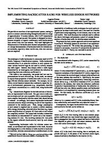
By combining equations (18) and (19), critical transmission and reception parameters are linked to detection probability. Next they will be linked to wireless sensor array formation. For the wireless sensor network, it has been assumed that signal detection using a single element is insufficient to meet requirements. Considering PD with unity signal to noise ratio as a boundary for a signal element reception, the probability of detection can be analyzed for increasing gain. Figure (2) demonstrates the resulting detection probabilities under various false alarm rate requirements. Note that this analysis ignores the ability of the array to diminish the effect of interferers from spatial geometry outside of the target beam.

Figure 2. Probability of detection versus gain for differing levels of receive antenna gain. Initial receive antenna gain is set at 2.15dBi – equivalent to a half wave dipole at resonance. SNR is set at unity for initial receiver antenna gain.

Clearly from figure (2), by increasing gain the probability of signal detection is increased. In a typical signal reception problem, increased gain may be realized by using a high gain antenna element or constructing an array of elements operating coherently. However, using wireless sensor nodes to detect and process an emitted signal presents a unique situation. A random deployment of nodes, as discussed in section (1), would not allow the use of a specified high gain element. At issue would be both the orientation of the beam pattern from the high gain element after deployment and the energy cost associated solely with that element node. Additionally, the disadvantages to having the high gain element associated with a central controller have been addressed previously. Therefore, using the power of beamforming in the array is the better alternative. Fixed fielded arrays do not have power limitations at each element. Further, aperture size is constant and known. Additionally, all elements tend to be active full time, providing highest available gain. In the wireless sensor case defined, there is a fundamental requirement to keep energy costs low and spread these costs over the network, as each node has a limited power supply. In order to apply the results of the Neyman-Pearson criterion under the energy constraints, the benefits of the randomly deployed sensor network may be used. Two useful relationships from literature are [10] N ∝G (20) 1 BW ∝ (21) D

5

Proceedings of the 42nd Hawaii International Conference on System Sciences - 2009

Where BW indicates main beam beamwidth, and D stands for aperture size. These proportional relationships are used as element spatial geometry is a major factor in gain and beamwidth determinations which must be accounted for in specific determination of these array attributes. The proposed methodology uses the relationship in equation (20), which states the number of array elements is generally proportional to array gain, to determine the initial size of a subset of the network nodes in order to meet gain requirements for detection. It will also be used to foster immediate demodulation when initial SNR is insufficient. The equation (21) relationship, which states the beamwidth of the main beam is inversely proportional to aperture size, is used to determine the number of simultaneous beam patterns required. Relating equation (20) to Neyman-Pearson, it must first be recognized that SNR is a function of N (written as SNR ( N ) ). This is true with other factors held constant and Gr varied by altering the number of participating nodes. Probability of detection can then be written directly.

(

PD = Q β 0 − SNR( N )

)

(22)

Exploiting this relationship is unique to the wireless sensor network problem. The density of sensor node deployment is critical in this array definition and on energy usage, as will be seen in section (4).

3. Detection and Follow-on Processing Methodology The proposed methodology for using a wireless sensor network as a radio frequency sensor array emphasizing initial probability of target signal detection is described as follows. Nodes are assumed deployed in a random fashion in the operating area such that K nodes are distributed over an area A . The nodes self organize and are in contact with a controlling station. Their locations are determined using location discovery techniques and are reported back to the controller.

3.1. Detection Array Set-up -- Step 1. The controller will determine a subarea, As , from the overall distribution area, A . -- Note 1. The dimensions of As will be dependent on desired beamwidth and gain of an array pattern in accordance with [6] and equations (20) and (21).

-- Note 2. For beamforming with random element distribution in a set aperture area, the beamwidth in any target direction is roughly the same [10]. Therefore, beams can be created for 360o coverage simultaneously in the central processor without additional messaging from the network nodes for each beam. As an example, a beamwidth of 45o can simultaneously form 16 beams overlapping roughly at their 3dB beamwidth points from a single input by the target elements. This is not exact, so overdetermination of the beams in processing may be required. -- Step 2. The nodes in the subarea, As , are used to form a signal detection array in accordance with the random array process in [6] and equation (7). -- Note 1. The number of nodes used to form an iteration of nodes, Pi , is determined based on the gain necessary to meet a required detection probability with a constraining false alarm rate. -- Note 2. Designating Λ N as the total number of nodes within As , it is assumed that Λ N  Pi such that multiple iteration runs can be made against a subarea of nodes before a new subarea is designated (assuming each node is used only once).

3.2. Post-detection Processing The post-detection process is shown in figure (3). Specific notes on this process follow. • The central controller has knowledge of which beam detects the signal, indicating a rough azimuth to the target. If multiple beams detect the signal, the central controller has information on which beam provided best signal to noise ratio • Follow-on actions by the array are based on user preference for action. • The detection process can continue in alternate beams during follow-on processing; however, the target signal may be regarded as an interferer for detection of other signals (frequency separation dependent). • When the number of nodes in an iteration, Pi , is increased for immediate demodulation, there is an associated increase in sensor energy usage. Therefore, this is used temporarily until the formal scheme can be assembled.

6

Proceedings of the 42nd Hawaii International Conference on System Sciences - 2009

per node are important. As a further cost consideration, the time for network reaction to a detected signal is of importance to operations. Clearly a network which saves energy but does not meet operational requirements due to time lag is not worth deploying. There are three important states to consider when evaluating energy usage in a sensor network. The transmit state indicates a node is active and transmitting collected data. The idle state indicates a node is active but waiting to transmit data. The sleep state indicates a minimal energy usage condition; however, there is additional energy expended in transitioning from a sleep state to idle. Basic quantities can be delineated to capture the energy costs associated with these states. Define δ as the energy cost per transmission (joules/transmission), χ1 as the energy expended when a node is on and waiting to transmit (joules), and χ 2 as the energy expended in waking up a node for operations and transmission. Because they tend to be smaller in magnitude, the quantities χ1 and

χ 2 are often considered as a percentage of δ . The energy expended to beamform the detection array, Γ D , Figure 3. Flow chart depicting post-detection processing for the wireless sensor network array.

4. Cost Analysis As noted in section (2), there are two specific assumptions related to energy cost in considering operations of this type of sensor network. • Expected signal of interest activity in the deployed region will be moderate. Therefore, extensive sleep periods for sensor nodes may not be available. • Dwell time of the array may be limited by either the battery life of the network nodes or by access times of the central controller. In this context, dwell time refers to the amount of time the array is available for operations. The first assumption conveys that the expected target signal activity will have an effect on detection strategy. Low activity periods may translate to a strategy that emphasizes network sleep. The second assumption goes to the heart of the major constraint for a wireless sensor network – the network is only available in full strength when power at the nodes is available. Therefore, energy usage in the network must be thrifty and spread as equitably among the nodes as possible. Based on these assumptions, costs in operating with the proposed methodology can be evaluated. Specifically, energy usage and spread of energy usage

is made up of energy to wake up nodes in As , Γ wake , energy while nodes sit idle, Γidle , and energy to transmit data to the controller, Γ xmit . Sleep energy will be ignored in this calculation, and will be throughout this section, as analysis is focused on energy use of the operating nodes. However, sleep energy must be included when assessing a projected lifetime of the network. Thus Γ D = Γ wake + Γidle + Γ xmit . (23) With the number of nodes in As known as Λ N , the first two addends can be quickly defined. Γ wake = Λ N χ 2 (24)

Γidle = ( Λ N − 1) χ1

(25)

As the process defined in [6] is used to provide a lowsidelobe array solution, the third addend from equation (23) can be defined where L indicates the number of iterations required to produce the desired array factor. L

Γ xmit = δ

¦P

i

(26)

i =1

Therefore, through simple substitution into equation (23), the energy required to operate the detection array in As , Γ D , can be explicitly defined. L

ΓD = δ

¦ P + (Λ i

N

− 1) χ1 + Λ N χ 2

(27)

i =1

This energy cost is then spread over the network as the subarea is redefined. It should be noted that the

7

Proceedings of the 42nd Hawaii International Conference on System Sciences - 2009

number of beams created for detection does not impact the energy cost. This is because beams are created in processing at the central controller using already collected data instead of through additional work by the element nodes. The central controller is not a contributing part of the sensor network; therefore, its energy usage not a concern. Post-detection processing not requiring additional node participation, including TDOA and LOB calculation, also does not require additional energy cost as node communication levels are not altered. However, increasing Pi and/or As for an adaptive beamforming solution after LOB determination or increasing Pi for immediate collection increase energy usage since additional nodes wake. As discussed in section (3), a detected signal may require additional receiver gain over the detection array for adequate collection. In general, an increase in gain can be linked to the number of elements in the beamforming solution, [10]. In order to sustain the array operations, an increase in the subarea Λ N may also be necessary when increasing Pi . (Note: The need to produce additional beams due to narrowing of the beamwidth with an increase in As is not an energy factor, as beams are processed in the central controller.) Designating the potentially increased factors with primes, the new energy cost can be written. L

Γ prime = δ

¦ P ' + (Λ i

N

'− 1) χ1 + Λ N ' χ 2

(28)

i =1

Figure (4) demonstrates the increase in energy costs under various constraints on Λ N . For this simulation, energy associated with transmission, idling, and waking up is assumed equal. Although this is not a realistic assumption, it does not affect the curve relationships. Additionally, an initial value for Λ N is chosen to provide a numeric solution. The figure shows a linear relationship between Pi and energy cost. The slope the curves varies due the increase in Λ N . A strict definition for the increase of Λ N necessary when increasing Pi would require specific knowledge of the deployment density. For the simulation, this increase is assumed linear associated with a uniform distribution. Although a Gaussian distribution may be more fitting for a random distribution, as discussed in [4], the distributions in the subarea can be described as uniform when they represent a small section of a much larger distribution. The density of sensor deployment is an important factor. In cases where Λ N does not require increase for increased Pi , the energy slope is more modest

during

active

beamforming.

Figure 4. Energy cost versus number of nodes in an iteration. The energy cost is constrained under various conditions with respect to the number of available nodes.

The detection process can continue using the higher gain array, or a subset of elements may be selected from the adaptive array inputs to maintain detection sensitivity. The increased energy cost is required until a decision occurs to cease signal demodulation (due to either operator determination or end of transmission). In order to facilitate immediate signal demodulation when the detection SNR is not adequate for this action, an increase in Pi without a corresponding increase in As can form a temporary solution until a TDOA/LOB/adaptive beamforming solution is available. Using the same prime notation, the temporary energy required can be defined. L

Γtemp = δ

¦ P ' + (Λ i

N

− 1) χ1 + Λ N χ 2

(29)

i =1

To demonstrate the energy usage of the proposed method, a comparison to the method in [8] is offered. In [8]’s method, all nodes with the exception of a local central controller are in sleep (conserving energy) prior to signal of interest detection. This has the benefit of extending network life during periods of target emitter inactivity. However, based on the assumption of moderate signal activity, of specific interest is energy usage during periods of active emitter operation. The comparison of methods during emitter operation is shown below in equation (30). The energy required in [8] is on the right hand side. This energy (taken from [8]) accounts for the energy required to wake up selected nodes, the energy from nodes in operating status but waiting to transmit, the energy from each

8

Proceedings of the 42nd Hawaii International Conference on System Sciences - 2009

transmission required to form the TDOA solution, and the energy required to beamform after a LOB is established. L

δ

¦ P + (Λ i

N

− 1) χ1 + Λ N χ 2