A Discriminative Graph-Based Parser for the Abstract Meaning Representation Jeffrey Flanigan
Sam Thomson Jaime Carbonell Chris Dyer Noah A. Smith Language Technologies Institute Carnegie Mellon University Pittsburgh, PA 15213, USA {jflanigan,sthomson,jgc,cdyer,nasmith}@cs.cmu.edu Abstract
Abstract Meaning Representation (AMR) is a semantic formalism for which a growing set of annotated examples is available. We introduce the first approach to parse sentences into this representation, providing a strong baseline for future improvement. The method is based on a novel algorithm for finding a maximum spanning, connected subgraph, embedded within a Lagrangian relaxation of an optimization problem that imposes linguistically inspired constraints. Our approach is described in the general framework of structured prediction, allowing future incorporation of additional features and constraints, and may extend to other formalisms as well. Our open-source system, JAMR, is available at: http://github.com/jflanigan/jamr
1
Introduction
Semantic parsing is the problem of mapping natural language strings into meaning representations. Abstract Meaning Representation (AMR) (Banarescu et al., 2013; Dorr et al., 1998) is a semantic formalism in which the meaning of a sentence is encoded as a rooted, directed, acyclic graph. Nodes represent concepts, and labeled directed edges represent the relationships between them–see Figure 1 for an example AMR graph. The formalism is based on propositional logic and neo-Davidsonian event representations (Parsons, 1990; Davidson, 1967). Although it does not encode quantifiers, tense, or modality, the set of semantic phenomena included in AMR were selected with natural language applications—in particular, machine translation—in mind. In this paper we introduce JAMR, the first published system for automatic AMR parsing. The
system is based on a statistical model whose parameters are trained discriminatively using annotated sentences in the AMR Bank corpus (Banarescu et al., 2013). We evaluate using the Smatch score (Cai and Knight, 2013), establishing a baseline for future work. The core of JAMR is a two-part algorithm that first identifies concepts using a semi-Markov model and then identifies the relations that obtain between these by searching for the maximum spanning connected subgraph (MSCG) from an edge-labeled, directed graph representing all possible relations between the identified concepts. To solve the latter problem, we introduce an apparently novel O(|V |2 log |V |) algorithm that is similar to the maximum spanning tree (MST) algorithms that are widely used for dependency parsing (McDonald et al., 2005). Our MSCG algorithm returns the connected subgraph with maximal sum of its edge weights from among all connected subgraphs of the input graph. Since AMR imposes additional constraints to ensure semantic well-formedness, we use Lagrangian relaxation (Geoffrion, 1974; Fisher, 2004) to augment the MSCG algorithm, yielding a tractable iterative algorithm that finds the optimal solution subject to these constraints. In our experiments, we have found this algorithm to converge 100% of the time for the constraint set we use. The approach can be understood as an alternative to parsing approaches using graph transducers such as (synchronous) hyperedge replacement grammars (Chiang et al., 2013; Jones et al., 2012; Drewes et al., 1997), in much the same way that spanning tree algorithms are an alternative to using shift-reduce and dynamic programming algorithms for dependency parsing.1 While a detailed 1
To date, a graph transducer-based semantic parser has not been published, although the Bolinas toolkit (http://www.isi.edu/publications/ licensed-sw/bolinas/) contains much of the necessary infrastructure.
words “New York City” can evoke the fragment represented by
want-01 ARG1 ARG0
(c / city :name (n / name :op1 "New" :op2 "York" :op3 "City"))))
visit-01
ARG0
ARG1
boy name op1 “New”
name op2
city
op3 “York”
“City”
(a) Graph. (w / want-01 :ARG0 (b / boy) :ARG1 (g / visit-01 :ARG0 b :ARG1 (c / city :name (n / name :op1 "New" :op2 "York" :op3 "City")))) (b) AMR annotation. Figure 1: Two equivalent ways of representing the AMR parse for the sentence, “The boy wants to visit New York City.”
comparison of these two approaches is beyond the scope of this paper, we emphasize that—as has been observed with dependency parsing—a diversity of approaches can shed light on complex problems such as semantic parsing.
2
Notation and Overview
Our approach to AMR parsing represents an AMR parse as a graph G = hV, Ei; vertices and edges are given labels from sets LV and LE , respectively. G is constructed in two stages. The first stage identifies the concepts evoked by words and phrases in an input sentence w = hw1 , . . . , wn i, each wi a member of vocabulary W . The second stage connects the concepts by adding LE -labeled edges capturing the relations between concepts, and selects a root in G corresponding to the focus of the sentence w. Concept identification (§3) involves segmenting w into contiguous spans and assigning to each span a graph fragment corresponding to a concept from a concept set denoted F (or to ∅ for words that evoke no concept). In §5 we describe how F is constructed. In our formulation, spans are contiguous subsequences of w. For example, the
We use a sequence labeling algorithm to identify concepts. The relation identification stage (§4) is similar to a graph-based dependency parser. Instead of finding the maximum-scoring tree over words, it finds the maximum-scoring connected subgraph that preserves concept fragments from the first stage, links each pair of vertices by at most one edge, and is deterministic2 with respect to a special set of edge labels L∗E ⊂ LE . The set L∗E consists of the labels ARG0–ARG5, and does not include labels such as MOD or MANNER, for example. Linguistically, the determinism constraint enforces that predicates have at most one semantic argument of each type; this is discussed in more detail in §4. To train the parser, spans of words must be labeled with the concept fragments they evoke. Although AMR Bank does not label concepts with the words that evoke them, it is possible to build an automatic aligner (§5). The alignments are used to construct the concept lexicon and to train the concept identification and relation identification stages of the parser (§6). Each stage is a discriminatively-trained linear structured predictor with rich features that make use of part-ofspeech tagging, named entity tagging, and dependency parsing. In §7, we evaluate the parser against goldstandard annotated sentences from the AMR Bank corpus (Banarescu et al., 2013) under the Smatch score (Cai and Knight, 2013), presenting the first published results on automatic AMR parsing.
3
Concept Identification
The concept identification stage maps spans of words in the input sentence w to concept graph fragments from F , or to the empty graph fragment ∅. These graph fragments often consist of just one labeled concept node, but in some cases they are larger graphs with multiple nodes and edges.3 2 By this we mean that, at each node, there is at most one outgoing edge with that label type. 3 About 20% of invoked concept fragments are multiconcept fragments.
Concept identification is illustrated in Figure 2 using our running example, “The boy wants to visit New York City.” Let the concept lexicon be a mapping clex : W ∗ → 2F that provides candidate graph fragments for sequences of words. (The construction of F and clex is discussed below.) Formally, a concept labeling is (i) a segmentation of w into contiguous spans represented by boundaries b, giving spans hwb0 :b1 , wb1 :b2 , . . . wbk−1 :bk i, with b0 = 0 and bk = n, and (ii) an assignment of each phrase wbi−1 :bi to a concept graph fragment ci ∈ clex (wbi−1 :bi ) ∪ ∅. Our approach scores a sequence of spans b and a sequence of concept graph fragments c, both of arbitrary length k, using the following locally decomposed, linearly parameterized function: Pk
>
f (wbi−1 :bi , bi−1 , bi , ci ) (1) where f is a feature vector representation of a span and one of its concept graph fragments in context. The features are: score(b, c; θ) =
i=1 θ
• Fragment given words: Relative frequency estimates of the probability of a concept graph fragment given the sequence of words in the span. This is calculated from the concept-word alignments in the training corpus (§5). • Length of the matching span (number of tokens). • NER: 1 if the named entity tagger marked the span as an entity, 0 otherwise. • Bias: 1 for any concept graph fragment from F and 0 for ∅. Our approach finds the highest-scoring b and c using a dynamic programming algorithm: the zeroth-order case of inference under a semiMarkov model (Janssen and Limnios, 1999). Let S(i) denote the score of the best labeling of the first i words of the sentence, w0:i ; it can be calculated using the recurrence: S(0) = 0 n o S(i) = max S(j) + θ > f (wj:i , j, i, c) j:0≤j g(e)
(2)
The features are shown in Table 1. Our solution to maximizing the score in Eq. 2, subject to the constraints, makes use of (i) an algorithm that ignores constraint 4 but respects the others (§4.1); and (ii) a Lagrangian relaxation that iteratively adjusts the edge scores supplied to (i) so as to enforce constraint 4 (§4.2). 4.1
Maximum Preserving, Simple, Spanning, Connected Subgraph Algorithm
The steps for constructing a maximum preserving, simple, spanning, connected (but not necessarily deterministic) subgraph are as follows. These steps ensure the resulting graph G satisfies the constraints: the initialization step ensures the preserving constraint is satisfied, the pre-processing step ensures the graph is simple, and the core algorithm ensures the graph is connected. 1. (Initialization) Let E (0) be the union of the concept graph fragments’ weighted, labeled, directed edges. Let V denote its set of vertices. Note that hV, E (0) i is preserving (constraint 4), as is any graph that contains it. It is also simple (constraint 4), assuming each concept graph fragment is simple. 2. (Pre-processing) We form the edge set E by including just one edge from ED between each pair of nodes: `
• For any edge e = u → − v in E (0) , include e in E, omitting all other edges between u and v.
• For any two nodes u and v, include only the highest scoring edge between u and v. Note that without the deterministic constraint, we have no constraints that depend on the label of an edge, nor its direction. So it is clear that the edges omitted in this step could not be part of the maximum-scoring solution, as they could be replaced by a higher scoring edge without violating any constraints. Note also that because we have kept exactly one edge between every pair of nodes, hV, Ei is simple and connected. 3. (Core algorithm) Run Algorithm 1, MSCG, on hV, Ei and E (0) . This algorithm is a (to our knowledge novel) modification of the minimum spanning tree algorithm of Kruskal (1956). Note that the directions of edges do not matter for MSCG. Steps 1–2 can be accomplished in one pass through the edges, with runtime O(|V |2 ). MSCG can be implemented efficiently in O(|V |2 log |V |) time, similarly to Kruskal’s algorithm, using a disjoint-set data structure to keep track of connected components.6 The total asymptotic runtime complexity is O(|V |2 log |V |). The details of MSCG are given in Algorithm 1. In a nutshell, MSCG first adds all positive edges to the graph, and then connects the graph by greedily adding the least negative edge that connects two previously unconnected components. Theorem 1. MSCG finds a maximum spanning, connected subgraph of hV, Ei Proof. We closely follow the original proof of correctness of Kruskal’s algorithm. We first show by induction that, at every iteration of MSCG, there exists some maximum spanning, connected subgraph that contains G(i) = hV, E (i) i: 6 For dense graphs, Prim’s algorithm (Prim, 1957) is asymptotically faster (O(|V |2 )). We conjecture that using Prim’s algorithm instead of Kruskall’s to connect the graph could improve the runtime of MSCG.
Name Label Self edge Tail fragment root Head fragment root Path Distance Distance indicators Log distance Bias
Description For each ` ∈ LE , 1 if the edge has that label 1 if the edge is between two nodes in the same fragment 1 if the edge’s tail is the root of its graph fragment 1 if the edge’s head is the root of its graph fragment Dependency edge labels and parts of speech on the shortest syntactic path between any two words in the two spans Number of tokens (plus one) between the two concepts’ spans (zero if the same) A feature for each distance value, that is 1 if the spans are of that distance Logarithm of the distance feature plus one. 1 for any edge.
Table 1: Features used in relation identification. In addition to the features above, the following conjunctions are used (Tail and Head concepts are elements of LV ): Tail concept ∧ Label, Head concept ∧ Label, Path ∧ Label, Path ∧ Head concept, Path ∧ Tail concept, Path ∧ Head concept ∧ Label, Path ∧ Tail concept ∧ Label, Path ∧ Head word, Path ∧ Tail word, Path ∧ Head word ∧ Label, Path ∧ Tail word ∧ Label, Distance ∧ Label, Distance ∧ Path, and Distance ∧ Path ∧ Label. To conjoin the distance feature with anything else, we multiply by the distance.
input : weighted, connected graph hV, Ei and set of edges E (0) ⊆ E to be preserved output: maximum spanning, connected subgraph of hV, Ei that preserves E (0) let E (1) = E (0) ∪ {e ∈ E | ψ > g(e) > 0}; create a priority queue Q containing {e ∈ E | ψ > g(e) ≤ 0} prioritized by scores; i = 1; while Q nonempty and hV, E (i) i is not yet spanning and connected do i = i + 1; E (i) = E (i−1) ; e = arg maxe0 ∈Q ψ > g(e0 ); remove e from Q; if e connects two previously unconnected components of hV, E (i) i then add e to E (i) end end return G = hV, E (i) i; Algorithm 1: MSCG algorithm.
Base case: Consider G(1) , the subgraph containing E (0) and every positive edge. Take any maximum preserving spanning connected subgraph M of hV, Ei. We know that such an M exists because hV, Ei itself is a preserving spanning connected subgraph. Adding a positive edge to M would strictly increase M ’s score without disconnecting M , which would contradict the fact that M is maximal. Thus M must contain G(1) . Induction step: By the inductive hypothesis, there exists some maximum spanning connected
subgraph M = hV, EM i that contains G(i) . Let e be the next edge added to E (i) by MSCG. If e is in EM , then E (i+1) = E (i) ∪ {e} ⊆ EM , and the hypothesis still holds. Otherwise, since M is connected and does not contain e, EM ∪ {e} must have a cycle containing e. In addition, that cycle must have some edge e0 that is not in E (i) . Otherwise, E (i) ∪ {e} would contain a cycle, and e would not connect two unconnected components of G(i) , contradicting the fact that e was chosen by MSCG. Since e0 is in a cycle in EM ∪ {e}, removing it will not disconnect the subgraph, i.e. (EM ∪{e})\ {e0 } is still connected and spanning. The score of e is greater than or equal to the score of e0 , otherwise MSCG would have chosen e0 instead of e. Thus, hV, (EM ∪ {e}) \ {e0 }i is a maximum spanning connected subgraph that contains E (i+1) , and the hypothesis still holds. When the algorithm completes, G = hV, E (i) i is a spanning connected subgraph. The maximum spanning connected subgraph M that contains it cannot have a higher score, because G contains every positive edge. Hence G is maximal. 4.2
Lagrangian Relaxation
If the subgraph resulting from MSCG satisfies constraint 4 (deterministic) then we are done. Otherwise we resort to Lagrangian relaxation (LR). Here we describe the technique as it applies to our task, referring the interested reader to Rush and Collins (2012) for a more general introduction to Lagrangian relaxation in the context of structured prediction problems. In our case, we begin by encoding a graph G = hVG , EG i as a binary vector. For each edge e in the fully dense multigraph D, we associate a bi-
nary variable ze = 1{e ∈ EG }, where 1{P } is the indicator function, taking value 1 if the proposition P is true, 0 otherwise. The collection of ze form a vector z ∈ {0, 1}|ED | . Determinism constraints can be encoded as a set of linear inequalities. For example, the constraint that vertex u has no more than one outgoing ARG0 can be encoded with the inequality: X X ARG0 1{u −−−→ v ∈ EG } = z ARG0 ≤ 1. u−−−→v v∈V
v∈V
All of the determinism constraints can collectively be encoded as one system of inequalities: Az ≤ b, with each row Ai in A and its corresponding entry bi in b together encoding one constraint. For the previous example we have a row Ai that has 1s in the columns corresponding to edges outgoing from u with label ARG0 and 0’s elsewhere, and a corresponding element bi = 1 in b. The score of graph G (encoded as z) can be written as the objective function φ> z, where φe = ψ > g(e). To handle the constraint Az ≤ b, we introduce multipliers µ ≥ 0 to get the Lagrangian relaxation of the objective function: Lµ (z) = maxz (φ> z + µ> (b − Az)), z∗µ = arg maxz Lµ (z).
L(z) is an upper bound on the unrelaxed objective function φ> z, and is equal to it if and only if the constraints Az ≤ b are satisfied. If L(z∗ ) = φ> z∗ , then z∗ is also the optimal solution to the constrained solution. Otherwise, there exists a duality gap, and Lagrangian relaxation has failed. In that case we still return the subgraph encoded by z∗ , even though it might violate one or more constraints. Techniques from integer programming such as branch-and-bound or cutting-planes methods could be used to find an optimal solution when LR fails (Das et al., 2012), but we do not use these techniques here. In our experiments, with a stepsize of 1 and max number of steps as 500, Lagrangian relaxation succeeds 100% of the time in our data. 4.3
In AMR, one node must be marked as the focus of the sentence. We notice this can be accomplished within the relation identification step: we add a special concept node root to the dense graph D, and add an edge from root to every other node, giving each of these edges the label FOCUS. We require that root have at most one outgoing FO CUS edge. Our system has two feature types for this edge: the concept it points to, and the shortest dependency path from a word in the span to the root of the dependency tree.
5
And the dual objective: L(z) = min Lµ (z), µ≥0
z∗ = arg maxz L(z). Conveniently, Lµ (z) decomposes over edges: Lµ (z) = maxz (φ> z + µ> (b − Az)) = maxz (φ> z − µ> Az) = maxz ((φ − A> µ)> z). So for any µ, we can find z∗µ by assigning edges the new Lagrangian adjusted weights φ − A> µ and reapplying the algorithm described in §4.1. We can find z∗ by projected subgradient descent, by starting with µ = 0, and taking steps in the direction: ∂Lµ ∗ − (z ) = Az∗µ . ∂µ µ If any components of µ are negative after taking a step, they are set to zero.
Focus Identification
Automatic Alignments
In order to train the parser, we need alignments between sentences in the training data and their annotated AMR graphs. More specifically, we need to know which spans of words invoke which concept fragments in the graph. To do this, we built an automatic aligner and tested its performance on a small set of alignments we annotated by hand. The automatic aligner uses a set of rules to greedily align concepts to spans. The list of rules is given in Table 2. The aligner proceeds down the list, first aligning named-entities exactly, then fuzzy matching named-entities, then date-entities, etc. For each rule, an entire pass through the AMR graph is done. The pass considers every concept in the graph and attempts to align a concept fragment rooted at that concept if the rule can apply. Some rules only apply to a particular type of concept fragment, while others can apply to any concept. For example, rule 1 can apply to any NAME concept and its OP children. It searches the sentence
for a sequence of words that exactly matches its OP children and aligns them to the NAME and OP children fragment. Concepts are considered for alignment in the order they are listed in the AMR annotation (left to right, top to bottom). Concepts that are not aligned in a particular pass may be aligned in subsequent passes. Concepts are aligned to the first matching span, and alignments are mutually exclusive. Once aligned, a concept in a fragment is never realigned.7 However, more concepts can be attached to the fragment by rules 8–14. We use WordNet to generate candidate lemmas, and we also use a fuzzy match of a concept, defined to be a word in the sentence that has the longest string prefix match with that concept’s label, if the match length is ≥ 4. If the match length is < 4, then the concept has no fuzzy match. For example the fuzzy match for ACCUSE -01 could be “accusations” if it is the best match in the sentence. WordNet lemmas and fuzzy matches are only used if the rule explicitly uses them. All tokens and concepts are lowercased before matches or fuzzy matches are done. On the 200 sentences of training data we aligned by hand, the aligner achieves 92% precision, 89% recall, and 90% F1 for the alignments.
6
Training
We now describe how to train the two stages of the parser. The training data for the concept identification stage consists of (X, Y ) pairs: • Input: X, a sentence annotated with named entities (person, organization, location, misciscellaneous) from the Illinois Named Entity Tagger (Ratinov and Roth, 2009), and part-ofspeech tags and basic dependencies from the Stanford Parser (Klein and Manning, 2003; de Marneffe et al., 2006). • Output: Y , the sentence labeled with concept subgraph fragments. The training data for the relation identification stage consists of (X, Y ) pairs: 7
As an example, if “North Korea” shows up twice in the AMR graph and twice in the input sentence, then the first “North Korea” concept fragment listed in the AMR gets aligned to the first “North Korea” mention in the sentence, and the second fragment to the second mention (because the first span is already aligned when the second “North Korea” concept fragment is considered, so it is aligned to the second matching span).
1. (Named Entity) Applies to name concepts and their opn children. Matches a span that exactly matches its opn children in numerical order. 2. (Fuzzy Named Entity) Applies to name concepts and their opn children. Matches a span that matches the fuzzy match of each child in numerical order. 3. (Date Entity) Applies to date-entity concepts and their day, month, year children (if exist). Matches any permutation of day, month, year, (two digit or four digit years), with or without spaces. 4. (Minus Polarity Tokens) Applies to - concepts, and matches “no”, “not”, “non.” 5. (Single Concept) Applies to any concept. Strips off trailing ‘-[0-9]+’ from the concept (for example run-01 → run), and matches any exact matching word or WordNet lemma. 6. (Fuzzy Single Concept) Applies to any concept. Strips off trailing ‘-[0-9]+’, and matches the fuzzy match of the concept. 7. (U.S.) Applies to name if its op1 child is united and its op2 child is states. Matches a word that matches “us”, “u.s.” (no space), or “u. s.” (with space). 8. (Entity Type) Applies to concepts with an outgoing name edge whose head is an aligned fragment. Updates the fragment to include the unaligned concept. Ex: continent in (continent :name (name :op1 "Asia")) aligned to “asia.” 9. (Quantity) Applies to .*-quantity concepts with an outgoing unit edge whose head is aligned. Updates the fragment to include the unaligned concept. Ex: distance-quantity in (distance-quantity :unit kilometer) aligned to “kilometres.” 10. (Person-Of, Thing-Of) Applies to person and thing concepts with an outgoing .*-of edge whose head is aligned. Updates the fragment to include the unaligned concept. Ex: person in (person :ARG0-of strike-02) aligned to “strikers.” 11. (Person) Applies to person concepts with a single outgoing edge whose head is aligned. Updates the fragment to include the unaligned concept. Ex: person in (person :poss (country :name (name :op1 "Korea"))) 12. (Goverment Organization) Applies to concepts with an incoming ARG.*-of edge whose tail is an aligned government-organization concept. Updates the fragment to include the unaligned concept. Ex: govern-01 in (government-organization :ARG0-of govern-01) aligned to “government.” 13. (Minus Polarity Prefixes) Applies to - concepts with an incoming polarity edge whose tail is aligned to a word beginning with “un”, “in”, or “il.” Updates the fragment to include the unaligned concept. Ex: - in (employ-01 :polarity -) aligned to “unemployment.” 14. (Degree) Applies to concepts with an incoming degree edge whose tail is aligned to a word ending is “est.” Updates the fragment to include the unaligned concept. Ex: most in (large :degree most) aligned to “largest.” Table 2: Rules used in the automatic aligner.
Split Train Dev. Test
• Input: X, the sentence labeled with graph fragments, as well as named enties, POS tags, and basic dependencies as in concept identification. • Output: Y , the sentence with a full AMR parse.8 Alignments are used to induce the concept labeling for the sentences, so no annotation beyond the automatic alignments is necessary. We train the parameters of the stages separately using AdaGrad (Duchi et al., 2011) with the perceptron loss function (Rosenblatt, 1957; Collins, 2002). We give equations for concept identification parameters θ and features f (X, Y ). For a sentence of length k, and spans b labeled with a sequence of concept fragments c, the features are: P f (X, Y ) = ki=1 f (wbi−1 :bi , bi−1 , bi , ci ) To train with AdaGrad, we process examples in the training data ((X 1 , Y 1 ), . . . , (X N , Y N )) one at a time. At time t, we decode (§3) to get Yˆ t and compute the subgradient: st = f (X t , Yˆ t ) − f (X t , Y t ) We then update the parameters and go to the next example. Each component i of the parameter vector gets updated like so: η θit+1 = θit − qP t
t0 t0 =1 si
sti
η is the learning rate which we set to 1. For relation identification training, we replace θ and f (X, Y ) in the above equations with ψ and P g(X, Y ) = e∈EG g(e). We ran AdaGrad for ten iterations for concept identification, and five iterations for relation identification. The number of iterations was chosen by early stopping on the development set.
7
Experiments
We evaluate our parser on the newswire section of LDC2013E117 (deft-amr-release-r3-proxy.txt). Statistics about this corpus and our train/dev./test splits are given in Table 3. 8
Because the alignments are automatic, some concepts may not be aligned, so we cannot compute their features. We remove the unaligned concepts and their edges from the full AMR graph for training. Thus some graphs used for training may in fact be disconnected.
Document Years 1995-2006 2007 2008
Sentences 4.0k 2.1k 2.1k
Tokens 79k 40k 42k
Table 3: Train/dev./test split.
P .92
Train R F1 .90 .91
P .90
Test R F1 .79 .84
Table 4: Concept identification performance.
For the performance of concept identification, we report precision, recall, and F1 of labeled spans using the induced labels on the training and test data as a gold standard (Table 4). Our concept identifier achieves 84% F1 on the test data. Precision is roughly the same between train and test, but recall is worse on test, implicating unseen concepts as a significant source of errors on test data. We evaluate the performance of the full parser using Smatch v1.0 (Cai and Knight, 2013), which counts the precision, recall and F1 of the concepts and relations together. Using the full pipeline (concept identification and relation identification stages), our parser achieves 58% F1 on the test data (Table 5). Using gold concepts with the relation identification stage yields a much higher Smatch score of 80% F1 . As a comparison, AMR Bank annotators have a consensus inter-annotator agreement Smatch score of 83% F1 . The runtime of our system is given in Figure 3. The large drop in performance of 22% F1 when moving from gold concepts to system concepts suggests that joint inference and training for the two stages might be helpful.
8
Related Work
Our approach to relation identification is inspired by graph-based techniques for non-projective syntactic dependency parsing. Minimum spanning tree algorithms—specifically, the optimum branching algorithm of Chu and Liu (1965) and Edmonds (1967)—were first used for dependency parsing by McDonald et al. (2005). Later ex-
concepts P gold .85 automatic .69
Train R F1 .95 .90 .78 .73
P .76 .52
Table 5: Parser performance.
Test R F1 .84 .80 .66 .58
average runtime (seconds) 0.0 0.1 0.2 0.3 0.4 0.5 0
10 20 30 40 sentence length (words)
Figure 3: Runtime of JAMR (all stages).
tensions allow for higher-order (non–edge-local) features, often making use of relaxations to solve the NP-hard optimization problem. Mcdonald and Pereira (2006) incorporated second-order features, but resorted to an approximate algorithm. Others have formulated the problem as an integer linear program (Riedel and Clarke, 2006; Martins et al., 2009). TurboParser (Martins et al., 2013) uses AD3 (Martins et al., 2011), a type of augmented Lagrangian relaxation, to integrate third-order features into a CLE backbone. Future work might extend JAMR to incorporate additional linguistically motivated constraints and higher-order features. The task of concept identification is similar in form to the problem of Chinese word segmentation, for which semi-Markov models have successfully been used to incorporate features based on entire spans (Andrew, 2006). While all semantic parsers aim to transform natural language text to a formal representation of its meaning, there is wide variation in the meaning representations and parsing techniques used. Space does not permit a complete survey, but we note some connections on both fronts. Interlinguas (Carbonell et al., 1992) are an important precursor to AMR. Both formalisms are intended for use in machine translation, but AMR has an admitted bias toward the English language. First-order logic representations (and extensions using, e.g., the λ-calculus) allow variable quantification, and are therefore more powerful. In recent research, they are often associated with combinatory categorial grammar (Steedman, 1996). There has been much work on statistical models for CCG parsing (Zettlemoyer and Collins, 2005; Zettlemoyer and Collins, 2007; Kwiatkowski et al., 2010, inter alia), usually using
chart-based dynamic programming for inference. Natural language interfaces for querying databases have served as another driving application (Zelle and Mooney, 1996; Kate et al., 2005; Liang et al., 2011, inter alia). The formalisms used here are richer in logical expressiveness than AMR, but typically use a smaller set of concept types—only those found in the database. In contrast, semantic dependency parsing—in which the vertices in the graph correspond to the words in the sentence—is meant to make semantic parsing feasible for broader textual domains. Alshawi et al. (2011), for example, use shift-reduce parsing to map sentences to natural logical form. AMR parsing also shares much in common with tasks like semantic role labeling and framesemantic parsing (Gildea and Jurafsky, 2002; Punyakanok et al., 2008; Das et al., 2014, inter alia). In these tasks, predicates are often disambiguated to a canonical word sense, and roles are filled by spans (usually syntactic constituents). They consider each predicate separately, and produce a disconnected set of shallow predicate-argument structures. AMR, on the other hand, canonicalizes both predicates and arguments to a common concept label space. JAMR reasons about all concepts jointly to produce a unified representation of the meaning of an entire sentence.
9
Conclusion
We have presented the first published system for automatic AMR parsing, and shown that it provides a strong baseline based on the Smatch evaluation metric. We also present an algorithm for finding the maximum, spanning, connected subgraph and show how to incorporate extra constraints with Lagrangian relaxation. Our featurebased learning setup allows the system to be easily extended by incorporating new feature sources.
Acknowledgments The authors gratefully acknowledge helpful correspondence from Kevin Knight, Ulf Hermjakob, and Andr´e Martins, and helpful feedback from Nathan Schneider, Brendan O’Connor, Waleed Ammar, and the anonymous reviewers. This work was sponsored by the U. S. Army Research Laboratory and the U. S. Army Research Office under contract/grant number W911NF-10-1-0533 and DARPA grant FA8750-12-2-0342 funded under the DEFT program.
References Hiyan Alshawi, Pi-Chuan Chang, and Michael Ringgaard. 2011. Deterministic statistical mapping of sentences to underspecified semantics. In Proc. of ICWS. Galen Andrew. 2006. A hybrid markov/semi-markov conditional random field for sequence segmentation. In Proc. of EMNLP. Laura Banarescu, Claire Bonial, Shu Cai, Madalina Georgescu, Kira Griffitt, Ulf Hermjakob, Kevin Knight, Philipp Koehn, Martha Palmer, and Nathan Schneider. 2013. Abstract meaning representation for sembanking. In Proc. of the Linguistic Annotation Workshop and Interoperability with Discourse. Shu Cai and Kevin Knight. 2013. Smatch: an evaluation metric for semantic feature structures. In Proc. of ACL. Jaime G. Carbonell, Teruko Mitamura, and Eric H. Nyberg. 1992. The KANT perspective: A critique of pure transfer (and pure interlingua, pure transfer, . . . ). In Proc. of the Fourth International Conference on Theoretical and Methodological Issues in Machine Translation: Empiricist vs. Rationalist Methods in MT. David Chiang, Jacob Andreas, Daniel Bauer, Karl Moritz Hermann, Bevan Jones, and Kevin Knight. 2013. Parsing graphs with hyperedge replacement grammars. In Proc. of ACL. Y. J. Chu and T. H. Liu. 1965. On the shortest arborescence of a directed graph. Science Sinica, 14:1396– 1400. Michael Collins. 2002. Discriminative training methods for hidden Markov models: Theory and experiments with perceptron algorithms. In Proc. of EMNLP. Dipanjan Das, Andr´e F. T. Martins, and Noah A. Smith. 2012. An exact dual decomposition algorithm for shallow semantic parsing with constraints. In Proc. of the Joint Conference on Lexical and Computational Semantics. Dipanjan Das, Desai Chen, Andr´e F. T. Martins, Nathan Schneider, and Noah A. Smith. 2014. Frame-semantic parsing. Computational Linguistics, 40(1):9–56. Donald Davidson. 1967. The logical form of action sentences. In Nicholas Rescher, editor, The Logic of Decision and Action, pages 81–120. Univ. of Pittsburgh Press. Marie-Catherine de Marneffe, Bill MacCartney, and Christopher D. Manning. 2006. Generating typed dependency parses from phrase structure parses. In Proc. of LREC.
Bonnie Dorr, Nizar Habash, and David Traum. 1998. A thematic hierarchy for efficient generation from lexical-conceptual structure. In David Farwell, Laurie Gerber, and Eduard Hovy, editors, Machine Translation and the Information Soup: Proc. of AMTA. Frank Drewes, Hans-J¨org Kreowski, and Annegret Habel. 1997. Hyperedge replacement graph grammars. In Handbook of Graph Grammars, pages 95– 162. World Scientific. John Duchi, Elad Hazan, and Yoram Singer. 2011. Adaptive subgradient methods for online learning and stochastic optimization. Journal of Machine Learning Research, 12:2121–2159, July. Jack Edmonds. 1967. Optimum branchings. National Bureau of Standards. Marshall L. Fisher. 2004. The Lagrangian relaxation method for solving integer programming problems. Management Science, 50(12):1861–1871. Arthur M Geoffrion. 1974. Lagrangean relaxation for integer programming. Springer. Daniel Gildea and Daniel Jurafsky. 2002. Automatic labeling of semantic roles. Computational Linguistics, 28(3):245–288. Jacques Janssen and Nikolaos Limnios. 1999. SemiMarkov Models and Applications. Springer, October. Bevan Jones, Jacob Andreas, Daniel Bauer, Karl Moritz Hermann, and Kevin Knight. 2012. Semantics-based machine translation with hyperedge replacement grammars. In Proc. of COLING. Rohit J. Kate, Yuk Wah Wong, and Raymond J. Mooney. 2005. Learning to transform natural to formal languages. In Proc. of AAAI. Dan Klein and Christopher D. Manning. 2003. Accurate unlexicalized parsing. In Proc. of ACL. Joseph B. Kruskal. 1956. On the shortest spanning subtree of a graph and the traveling salesman problem. Proc. of the American Mathematical Society, 7(1):48. Tom Kwiatkowski, Luke Zettlemoyer, Sharon Goldwater, and Mark Steedman. 2010. Inducing probabilistic CCG grammars from logical form with higherorder unification. In Proc. of EMNLP. Percy Liang, Michael I. Jordan, and Dan Klein. 2011. Learning dependency-based compositional semantics. In Proc. of ACL. Andr´e F. T. Martins, Noah A. Smith, and Eric P. Xing. 2009. Concise integer linear programming formulations for dependency parsing. In Proc. of ACL.
Andr´e F. T. Martins, Noah A. Smith, Pedro M. Q. Aguiar, and M´ario A. T. Figueiredo. 2011. Dual decomposition with many overlapping components. In Proc. of EMNLP. Andr´e F. T. Martins, Miguel Almeida, and Noah A. Smith. 2013. Turning on the turbo: Fast third-order non-projective Turbo parsers. In Proc. of ACL. Ryan Mcdonald and Fernando Pereira. 2006. Online learning of approximate dependency parsing algorithms. In Proc. of EACL, page 81–88. Ryan McDonald, Fernando Pereira, Kiril Ribarov, and Jan Hajiˇc. 2005. Non-projective dependency parsing using spanning tree algorithms. In Proc. of EMNLP. Terence Parsons. 1990. Events in the Semantics of English: A study in subatomic semantics. MIT Press. Robert C. Prim. 1957. Shortest connection networks and some generalizations. Bell System Technology Journal, 36:1389–1401. Vasin Punyakanok, Dan Roth, and Wen-tau Yih. 2008. The importance of syntactic parsing and inference in semantic role labeling. Computational Linguistics, 34(2):257–287. Lev Ratinov and Dan Roth. 2009. Design challenges and misconceptions in named entity recognition. In Proc. of CoNLL. Sebastian Riedel and James Clarke. 2006. Incremental integer linear programming for non-projective dependency parsing. In Proc. of EMNLP. Frank Rosenblatt. 1957. The perceptron–a perceiving and recognizing automaton. Technical Report 85460-1, Cornell Aeronautical Laboratory. Alexander M. Rush and Michael Collins. 2012. A tutorial on dual decomposition and Lagrangian relaxation for inference in natural language processing. Journal of Artificial Intelligence Research, 45(1):305—-362. Mark Steedman. 1996. Surface structure and interpretation. Linguistic inquiry monographs. MIT Press. John M. Zelle and Raymond J. Mooney. 1996. Learning to parse database queries using inductive logic programming. In Proc. of AAAI. Luke S. Zettlemoyer and Michael Collins. 2005. Learning to map sentences to logical form: Structured classification with probabilistic categorial grammars. In Proc. of UAI. Luke S. Zettlemoyer and Michael Collins. 2007. Online learning of relaxed CCG grammars for parsing to logical form. In In Proc. of EMNLP-CoNLL.