A Comparison of Capital Budgeting Techniques

Capital budgeting deals with setting the criteria and prescribing the process required for making capital investment choices. Choosing an investment project, that is, making a capital investment choice is ultimately a cost/benefit analysis. It requires valuing the project by comparing the payoff to its costs.

Problem Value, rank and select investment projects

Example 1. Required rate year 1: year 2 year 3 year 4 year 5 Initial Cost

Project A

Project B

Project C

7.7% $400 $1,250 $900.00 $3,000.00 $1,000 $5,045

3% $100.00 $200 $150.00 $100 $50 $490.67

6% $5,200 $4,000 $1,000 $200 $100 $9,687.23

1

Capital Budgeting Techniques A collection of methods allowing the manager to choose among a variety of investment projects. Methods: • • • • • • •

Average Accounting Return Payback Discounted payback Internal Rate of Return Modified Internal Rate of Return Net Present Value Profitability Index

Average Accounting Return (AAR) AAR is the ratio of the Average Net Income to the Average Book Value. Decision rule: Take the project if AAR is greater than some target ratio set by accountants. Disadvantages: It has too many flaws, don't ever use it. Payback period Payback is the time it takes to recover the initial cost of the investment. Payback is usually measured in years. Decision rule: Take the project with the shortest payback period Disadvantages It ignores time value of money It ignores risk It ignores cash inflows beyond the cutoff point Project A: Payback calculation Period

Cash flow

Amount left to recover

0

-$5,045.00

-$5,045.00

1

$400

$4,645.00

2

$1,250

$3,395.00

3

$900.00

$2,495.00

0.83

$3,000.00

$0.00

Notice that in the fourth year, there is $2,495 left to recuperate, and the annual cash flow equals $3,000 2

Obviously, $2,495/$3,000 = 0.83 Payback here is interpreted as follows: It takes between three and four years to recuperate the initial cost of the project. Project B: Payback calculation Period

Cash flow

Amount left to recover

0

-$490.67

-$490.67

1

$100.00

$390.67

2

$200

$190.67

3

$150.00

$40.67

0.41

$100

$0.00

The payback period of project B is also between three and four years (3.41 years) Notice that $40.67/$100 = 0.41 (approximately)

Project C: Payback calculation Period

Cash flow

Amount left to recover

0

-$9,687.23

-$9,687.23

1

$5,200

$4,487.23

2

$4,000

$487.23

0.49

$1,000

$0.00

The payback of project C is 2.49 years. Notice that $487.23/$1,000 = 0.49 (approximately) Ranking: 1. project C: 2.49 years 2. project B: 3.41 years 3. project A: 3.83 years All three projects are viable, but project C is the first to recover its initial cost.

3

Discounted payback period (DPB) DPB is the time it takes to recover the initial cost of the investment. Payback uses nominal CF; DPB uses discounted CF Decision rule: Take the project with the shortest discounted payback period. Disadvantages: DPB ignores cash inflows beyond the cutoff point The calculation of discounted payback is exactly the same as that of payback, except that instead of using nominal cash flow, we use present values instead. Project A: Discounted payback calculation Period

Cash flow at 7.7%

Amount left to recover

0

-$5,045.00

-$5,045.00

1

$371.40

$4,673.60

2

$1,077.65

$3,595.95

3

$720.44

$2,875.51

4

$2,229.76

$645.75

0.94

$690.12

0

The discounted payback of project A is just under 5 years (4.94) Notice that $645.75/$690.12 = 0.94

Project B: Discounted payback calculation Period

Cash flow at 3%

Amount left to recover

0

-$490.67

-$490.67

1

$97.09

$393.58

2

$188.52

$205.06

3

$137.27

$67.79

0.76

$88.85

$0.00

The discounted payback of project B is just under 4 years (3.76) Notice that $67.79/$88.85 = 0.76

4

Project C: Discounted payback calculation Period

Cash flow at 6%

Amount left to recover

0

-$9,687.23

-$9,687.23

1

$4,905.66

$4,781.57

2

$3,559.99

$1,221.58

3

$839.62

$381.96

4

$158.42

$223.55

5

$74.73

$148.82

Notice that the project never recovers its initial cost. At the end of year 5 there is still $148.82 left.

5

Internal Rate of Return IRR is the discount rate that makes the present value of the project equal to its initial cost. Decision rule: Take the project If the IRR exceeds the required rate of return Disadvantages: • Reinvestment rate assumption is unrealistic • Multiple IRR • IRR cannot rank mutually exclusive projects Calculation Project A: Set: Initial cost (A) = PV(project A): $5,045 = $400/(1+IRR) + $1,250/(1+IRR)2 + $900/(+IRR)3 + $3,000/(1+IRR)4 + $1,000/(1+IRR)5 IRR(A) = 8% Since IRR(A) > 7.7%, accept project (A)

Project B: $490.67 = $100/(1+IRR) + $400/(1+IRR)2 + $150/(1+IRR)3 + $100/(1+IRR)4 + $50/(1+IRR)5 IRR(B) = 8% Since IRR(B) > 3%, accept project B

Project C: $9,687.23=$5,200/(1+IRR) + $4,000/(1+IRR)2 + $1,000/(1+IRR)3 + $200/(1+IRR)4 + $100/(1+IRR)5 IRR(C) = 5%. Since IRR(C) < 6%, reject project C

6

Modified Internal Rate of Return MIRR is the discount rate that makes the future value of the project equal the future value of the initial cost. MIRR requires a reinvestment rate. Decision rule: Take the project if MIRR is larger than the required rate. Disadvantages: MIRR cannot rank mutually exclusive projects. MIRR calculation Project A: Let us assume the reinvestment rate is 5%. Set the future value of project's cash flow at 5%. The time horizon, i.e. number of periods, will equal the duration of the project. FV(CF at 5%) = $400(1.05)4 + $1,250(1.05)3 + $900(1.05)2 + $3,000(1.05) + $1,000 On the other hand, the FV of the initial cost compounded at MIRR is: FV (initial cost) = $5,045(1+MIRR)5 Obviously, MIRR is unknown at this stage, and this is precisely the quantity we want to find. To do so we need to solve the equation: $400(1.05)4 + $1,250(1.05)3 + $900(1.05)2 + $3,000(1.05) + $1,000 = $5,045(1+MIRR(A))5 Using elementary algebra, we find that: MIRR(A)= ([ $400(1.05)4 + $1,250(1.05)3 + $900(1.05)2 + $3,000(1.05) + $1,000]/$5,045)1/5 - 1 MIRR(A) = 7% Since MIRR is less than 7.7% (the required rate of return for A), we must reject project A. For project B: FV(CF at 5%) = $100(1.05)4 + $200(1.05)3 + $150(1.05)2 + $100(1.05) + $50 FV (initial cost) = $490.67(1+MIRR(B))5 $100(1.05)4 + $200(1.05)3 + $150(1.05)2 + $1001.05) + $50 = $490.67(1+MIRR(B))5 MIRR(B) = 6.54% Since MIRR is more than 3% (the required rate of return for B), we should accept project B. Project C: FV(CF at 5%) = $5,200(1.05)4 + $4,000(1.05)3 + $1,000(1.05)2 + $200(1.05) + $100 FV (initial cost) = $9,687.23(1+MIRR(C))5 $5,200(1.05)4 + $4,000(1.05)3 + $1,000(1.05)2 + $2001.05) + $100 = $9,687.23(1+MIRR(C))5 MIRR(C) = 5% Since MIRR is less than 6% (the required rate of return for C), we must reject project C. Only is B viable, given a reinvestment rate of 5% 7

Net Present Value Net Present Value is the difference between the present value of a project and its initial cost: NPV= Present value - Initial Cost Decision rule: If NPV is positive, take the project. Disadvantages: Very complex analysis, too many variables to forecast, as it will be seen later. Calculation: In order to calculate NPV, we must first estimate the PV of total cash flows; then we subtract the initial cost of the project. Project A: PV(A) =$400/(1.077) + $1,250/(1.077)2 + $900/(1.077)3 + $3,000/(1.077)4 + $1,000/(1.077)5 Initial cost (A) = $5,045 NPV(A) = $44.36 Project B: PV(B) =$100/(1.03) + $400/(1.03)2 + $150/(1.03)3 + $100/(1.03)4 + $50/(1.03)5 Initial cost (B) = $490.67 NPV (B) = $64.2 Project C: PV(C) =$5,200/(1.06) + $4,000/(1.06)2 + $1,000/(1.06)3 + $200/(1.06)4 + $100/(1.06)5 Initial cost (C) = $9,687.23 NPV (C) = -$148.81 Corollary: When Required Rate = IRR, then NPV = 0 Remember that IRR is the discount rate that makes the PV of the project equal its initial cost. In other words, IRR is the rate that makes the NPV of the project equal to zero. If still not convinced, consider the present value of our projects at the IRR. If the discount rate is equal to 8%, NPV(A) = $400/(1.08) + $1,250/(1.08)2 + $900/(1.08)3 + $3,000/(1.08)4 + $1,000/(1.08)5 - $5,045 NPV(A) = 0 When the discount rate equals 8%: NPV(B) = $100/(1.08) + $400/(1.08)2 + $150/(1.08)3 + $100/(1.08)4 + $50/(1.08)5 - $490.67 NPV(B) = 0 When the discount rate equals 5%: NPV(C) = $5,200/(1.05) + $4,000/(1.05)2 + $1,000/(1.05)3 + $200/(1.05)4 + $100/(1.05)5 - $9,687.23 NPV(C) = 0

8

The Profitability Index The profitability index is the ratio of project PV to initial cost PI = PV/Initial cost Decision rule: Take the project if PI > 1 Disadvantages PI cannot rank mutually exclusive projects. PI calculation Project A: PI(A) = PV(A)/Initial cost = 5,089.36/$5,045 PI(A) = $400/(1.077) + $1,250/(1.077)2 + $900/(1.077)3 + $3,000/(1.077)4 + $1,000/(1.077)5/$5,045 PI(A) = 1.0088 Project B: PI(B) = $100/(1.03) + $400/(1.03)2 + $150/(1.03)3 + $100/(1.03)4 + $50/(1.03)5 /$490.67 PI(B) = 1.131 Project C: PI(C) = $5,200/(1.06) + $4,000/(1.06)2 + $1,000/(1.06)3 + $200/(1.06)4 + $100/(1.06)5 /$9,687.23 PI(C) = 0.9846 Only A and B are viable

Why can’t PI rank the projects? Consider the following example: Present value Initial cost PI NPV

Project x

Project y

$25,000,000 $24,000,000 1.042 $1,000,000

$3,000 $1,000 3 $2,000.00

PI(x) < PI(y)‫‏‬ but NPV(x) > NPV(y)‫‏‬ In project valuation, measures of absolute wealth are more appropriate than measures of relative efficiency. 9

Summary: The results of our capital budgeting techniques are summarized below.

Required rate Cost Present value Future value (5%) Payback period Discounted payback IRR MIRR Net present value Profitability index

Project A:

Project B:

Project C:

7.7% $5,045 $5,089.36 $7,075.45 3.83 years 4.94 years 8.00% 7.00% $44.36 1.01

3% $490.67 $554.84 $673.45 3.41 years 3.76 years 8.00% 6.54% $64.20 1.13

6% $9,687.23 9,538.42 $12,363.5 2.49 years N/A 5% 5% -$148.81 0.9846

10

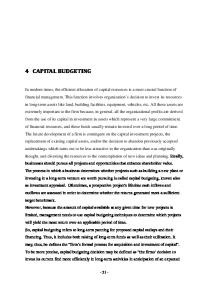
NPV profiles

NPV profiles are graphs showing the relationship between discount rates and NPV. For projects with conventional cash flows, this relationship is usually downward sloping; that is, as the discount rate increases, NPV is decreasing. NPV profiles are especially useful when all projects have the same required rate of return, or when the discount rate is hard to ascertain.

NPV Profiles

$2,000.00 $1,500.00 $1,000.00 $500.00 $0.00 -$500.00 NPV ($) -$1,000.00 -$1,500.00 -$2,000.00 -$2,500.00 -$3,000.00 0.00%

5.00%

10.00%

15.00%

20.00%

NPV (A)

11

25.00% Discount rate (%)

NPV (B)

NPV (C)

30.00%

What are the discount rates at which we are indifferent among those three projects? We have to find the point where all three profiles intersect at the same time. Following a casual inspection of the NPV profiles, it is not hard to see that they do not intersect. There is no rate at which the NPV of all three is the same. At least, we can search for the discount rate that makes us indifferent between project A and B. This amounts to finding the rate at which NPV(A) = NPV(B) Set: NPV(A) = NPV(B) and solve for the discount rate, that is: $400/(1+r) + $1,250/(1+r)2 + $900/(+r)3 + $3,000/(1+r)4 + $1,000/(1+r)5 - $5,045 = = $100/(1+r) + $400/(1+r)2 + $150/(1+r)3 + $100/(1+r)4 + $50/(1+r)5 - $490.67 Using elementary algebra, or trial-and-error (more likely), we find that the NPVs of the two projects are equal when r = 8% (approximately). At any rate below 8% for both projects project A is better. Beyond 8% both projects have negative NPVs. What is the discount rate that makes us indifferent between project A and C? This amounts to finding the rate at which NPV(A) = NPV(C) $400/(1+r) + $1,250/(1+r)2 + $900/(+r)3 + $3,000/(1+r)4 + $1,000/(1+r)5 - $5,045 = = $5,200/(1+r) + $4,000/(1+r)2 + $1,000/(1+r)3 + $200/(1+r)4 + $100/(1+r)5 -$9,687.23 It is not hard to see that for any discount rate within a reasonable range (that is 0 to 100%) there is no solution to this equation. The NPV profile of project A and C never meet. We will always prefer A over C regardless of the discount rate, because the profile of A is always above that of C. What is the discount rate that makes us indifferent between project B and C? This amounts to finding the rate at which NPV(B) = NPV(C) $100/(1+r) + $400/(1+r)2 + $150/(1+r)3 + $100/(1+r)4 + $50/(1+r)5 - $490.67 = $5,200/(1+r) + $4,000/(1+r)2 + $1,000/(1+r)3 + $200/(1+r)4 + $100/(1+r)5 -$9,687.23 Using elementary algebra, or trial-and-error, we find r = 4.75% (approximately). Between 0 and 4.75% for both projects, C is always preferred over B. For discount rates above 4.75%, up to 8%, B is always preferred over C.

12

A summary of NPV profiles Range of discount Significance of rates upper bound

Project A

Project B

0 to 4.75%

Crossover between B&C

Accept

Accept Accept (marginally)

A, C, B

4.75% to 5%

IRR(C)

Accept

Accept Accept (marginally)

A, B, C

5% to 8%

IRR (A), IRR (B) and crossover between A & B

Accept

Accept Reject (marginally)

A, B, C

Reject

Reject

B, A, C

8% and beyond

13

Project C

reject

Ranking

Example 2 Consider the following cash flows: Period

Cash flow A

Cash flow B

Cash flow C

0 1 2 3 4 5 6 7

-$1,600.00 $0.00 $0.00 $400.00 $400.00 $400.00 $400.00 $400.00

-$451.00 $100.00 $200.00 $150.00 $100.00 $50.00

-$503.99 $2,862.00 -$6,070.00 $5,700.00 -$2,000.00

Discount rate Reinvestment rate

4.60% 3.00%

3.00% 10.00%

66.90% 10.00%

Payback Discounted payback IRR MIRR NPV PI Projects A and B are nice, clean, and comforting conventional projects; project C has alternating sign cash flow, which spells trouble. As will see, the estimation and interpretation of the IRR is more problematic, but luckily we can always fall back on MIRR and NPV, especially NPV.

14

Payback Project A: Discounted payback calculation Period

Cash flow

Amount left to recover

0

-$1,600.00

-$1,600.00

1

$0.00

$1,600.00

2

$0.00

$1,600.00

3

$400.00

$1,200.00

4

$400.00

$800.00

5

$400.00

$400.00

6

$400.00

$0.00

The payback of project A is exactly 6 years Project B: Discounted payback calculation Period

Cash flow

Amount left to recover

0

-$451.00

-$451.00

1

$100.00

$351.00

2

$200.00

$151.00

3

$150.00

$1.00

0.01

$100.00

$0.00

The discounted payback of project B is 3 years (3.01) Project C has cash flow with alternating signs. The initial cost is recovered after the first year, but subsequent negative cash outflows make the estimation of payback less meaningful.

15

Discounted payback Project A: Discounted payback calculation Period

Cash flow at 4.60%

Amount left to recover

0

-$1,600.00

-$1,600.00

1

$0.00

$1,600.00

2

$0.00

$1,600.00

3

$349.51

$1,250.49

4

$334.14

$916.34

5

$319.45

$596.89

6

$305.40

$291.49

7

$291.97

$0.00

The payback of project A is exactly 7 years Project B: Discounted payback calculation Period

Cash flow at 3%

Amount left to recover

0

-$451.00

-$451.00

1

$97.09

$353.91

2

$188.52

$165.39

3

$137.27

$28.12

0.32

$88.85

$0.00

The discounted payback of project B is years (3.32). notice that $28.12/$88.85 = 0.32 Project C has cash flow with alternating signs. Again, estimating the discounted payback is a rather not an insightful exercise.

16

Internal Rate of Return Project A: $1,600 = $400/(1+IRR)3 + $400/(1+IRR)4 + $400/(1+IRR)5 + $400/(1+IRR)6 + $400/(1+IRR)7 Using trial and error we find that the IRR(A) is approximately 4.6%, virtually equal to the required rate.

Project B $451 = $100/(1+IRR) + $200/(1+IRR)2 + $150/(1+IRR)3 + $100/(1+IRR)4 + $50/(1+IRR)5 Using trial and error we find that the IRR(B) is approximately 11.7%, larger than the required rate. Project C $503.99 = $2,862/(1+IRR) - $6,070/(1+IRR)2 + $5,700/(1+IRR)3 - $2,000/(1+IRR)4 Using trial and error we find two internal rates: One at approximately 24.1% and the other one at 66.9%, virtually equal to the required rate. There are two more rates, but we do not bother with them since they must be outside of any reasonable range. What significance would a negative, or a positive but large rate could add to an already ambiguous situation. How do we interpret the results? The answer will become clear when discussing NPV profiles. Modified internal rate of return Project A: $1,600(1+MIRR)7 = $400(1.03)4 + $400(1.03)3 + $400(1.03)2 + $400/(1.03) + $400 We find that the MIRR(A) is approximately 4.13%

Project B $451(1+MIRR)5 = $100(1.1)4 + $200(1.1)3 + $150/(1.1)2 + $100(1.1) + $50 We find that the MIRR(B) is approximately 10.8%, larger than the required rate, yet smaller than the IRR, simply because reinvestment was made at a rate lower than 11.7% Project C $503.99(1+MIRR)4 = $2,862(1.1)3 - $6,070(1.1)2 + $5,700(1.1) - $2,000 We find that the MIRR(C) is approximately 9.9%

17

Net Present Value Project A NPV(A) = -$1,600 + $400/(1.046)3 + $400/(1.046)4 + $400/(1.046)5 + $400/(1.046)6 + $400/(1.046)7 NPV(A) = $0.48 Project B NPV(B) = -$451 + $100/(1.03) + $200/(1.03)2 + $150/(1.03)3 + $100/(1.03)4 + $50/(1.03)5 NPV(B) = $103.86 Project C NPV(C) = -$503.99 + $2,862/(1.67) - $6,070/(1.67)2 + $5,700/(1.67)3 - $2,000/(1.67)4 NPV(C) = 0

Profitability index PI(A) = [$400/(1.046)3 + $400/(1.046)4 + $400/(1.046)5 + $400/(1.046)6 + $400/(1.046)7 ]/$1,600 PI(A) = 1

PI(B) = [$100/(1.03) + $200/(1.03)2 + $150/(1.03)3 + $100/(1.03)4 + $50/(1.03)5]/$451 PI(B) = 1.23 PI(C) = [$2,862/(1.67) - $6,070/(1.67)2 + $5,700/(1.67)3 - $2,000/(1.67)4]/$503.99 PI(C) = 1

18

Summary of several capital budgeting methods. Period

Cash flow A

Cash flow B

Cash flow C

0 1 2 3 4 5 6 7

-$1,600.00 $0.00 $0.00 $400.00 $400.00 $400.00 $400.00 $400.00

-$451.00 $100.00 $200.00 $150.00 $100.00 $50.00

-$503.99 $2,862.00 -$6,070.00 $5,700.00 -$2,000.00

Discount rate Reinvestment rate

4.60% 3.00%

3.00% 10.00%

66.90% 10.00%

Payback Discounted payback IRR MIRR NPV PI

6 7

3.01 3.32

na. na.

4.60% 4.13% $0.48 1.00

11.70% 10.83% $103.86 1.23

24.10% & 67.00% 9.90% $0.00 1.00

In this example, for the given combination of discount rates and cash flows, project B clearly dominates the other two projects. Although project A's NPV is marginally positive, the project represents a questionable choice. The same goes for project C. A zero net present value makes us indifferent between accepting and rejecting the project, that is, in theory. Without other extra-monetary considerations, it is hard to justify taking on a project that offers no obvious benefits.

19

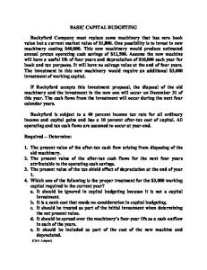
NPV Profiles

$600.00 $400.00 $200.00 $0.00 -$200.00 -$400.00 NPV ($) -$600.00 -$800.00 -$1,000.00 -$1,200.00 0.00%

5.00%

10.00%

15.00%

20.00%

25.00%

30.00% Discount rate (%)

NPV (A)

20

NPV (B)

NPV (C)

Crossover rate between Projects A and B Period

Cash flow A

Cash flow B

A-B

0 1 2 3 4 5 6 7

-$1,600.00 $0.00 $0.00 $400.00 $400.00 $400.00 $400.00 $400.00

-$451.00 $100.00 $200.00 $150.00 $100.00 $50.00 $0.00 $0.00

-$1,149 -$100 -$200 $250 $300 $350 $400 $400

In order to find the crossover rate between projects A and B, we need to estimate the discount rate that makes the present value of the difference in the cash flow between the two projects equal to zero. In other words we take the difference in cash flow between the two projects and we estimate the IRR. In the equation below, r is the crossover rate between projects A and B: -$1,149-$100/(1+r) -$200/(1+r)2+$250/(1+r)3 + $300/(1+r)4 +$350/(1+r)5 +$400/(1+r)6 +$400(1+r)7 =0 Using trial and error we find that r is approximately equal to 3.35%. At rates between 0 and 3.35%, project A ranks better than project B, that is, it has a higher net present value. Beyond 3.35%, project B ranks better than project A.

Crossover rate between projects A and C Period Cash flow A 0 1 2 3 4 5 6 7

-$1,600.00 $0.00 $0.00 $400.00 $400.00 $400.00 $400.00 $400.00

Cash flow C

A-C

-$503.99 $2,862.00 -$6,070.00 $5,700.00 -$2,000.00 $0.00 $0.00 $0.00

-$1,096 -$2,862.00 $6,070.00 -$5,300.00 $2,400.00 $400.00 $400.00 $400.00

In the equation below, r is the crossover rate between projects A and C: -$1,096-$2,862/(1+r)+$6,070/(1+r)2-$5,300/(1+r)3 +$2,400/(1+r)4 +$400/(1+r)5 +$400/(1+r)6 +$400/ (1+r)7 =0 Using trial and error, we find the crossover rate between projects A and B approximately equal to 4.67%. Between zero and 4.67%, Project A ranks better than project C, that is, it has a higher net present value. Beyond 4.67%, project C ranks better than A.

21

Crossover rate between projects B and C Period Cash flow B 0 1 2 3 4 5

-$451.00 $100.00 $200.00 $150.00 $100.00 $50.00

Cash flow C

B-C

-$503.99 $2,862.00 -$6,070.00 $5,700.00 -$2,000.00 $0.00

$52.99 -$2,762.00 $6,270.00 -$5,550.00 $2,100.00 $50.00

In the equation below, r is the crossover rate between projects B and C: $52.99-$2,762/(1+r)+$6,270/(1+r)2-$5,550/(1+r)3 +$2,100/(1+r)4 +$50/(1+r)5 =0 Using trial and error, we find the crossover rate between projects B and C approximately equal to 11.8%. Between zero and 11.8%, Project B ranks better than project C, that is, it has a higher net present value. Beyond 11.8%, project C ranks better than B.

A summary of NPV profiles Range of discount Significance of rates upper bound

Project A

Project B

Project C

Ranking

0 to 3.35%

Crossover between A&B

Accept

Accept

Reject

A, B, C

3.35% to 4.6%

IRR(A)

Accept

Accept

Reject

B, A, C

4.6% to 4.67%

Crossover between A&C

Reject

Accept

Reject

B, A, C

4.67% to 11.7%

IRR(B)

Reject

Accept

Reject

B, C, A

11.7% to 11.8%

Crossover between B&C

Reject

Reject

Reject

B, C, A

11.8% to 24.1%

IRR(C)1

Reject

Reject

Reject

C, B, A

24.1% to 67%

IRR(C)2

Reject

Reject

Accept (marginally)

C, B, A

Reject

Reject

Reject

C, B, A

67% and beyond

22

Example 3 Consider the following three projects: Period 0 1 2 3 4 5

Cash flow A -$1,600.00 $1,600.00

Cash flow B $500 $0 -$400

Cash flow C $500 -$500 $500 -$500 $500 -$500

Discount rate Reinvestment

30.00% 3.00%

11.00% 0.00%

30.00% 10.00%

Payback Discounted payback IRR MIRR NPV PI

The three projects have again different lives and unconventional cash flows, which makes comparison and evaluation a little trickier.

23

Project A Payback: It is obviously one year, no need to engage in redundant calculations. Discounted payback: As long as the discount rate is larger than zero, the project will never pay back, since the PV of $1,600 will always be less than $1,600 IRR: $1,600 = $1,600/(1+IRR) The PV of $1,600 is equal to $1,600 only when the discount rate is zero, hence IRR = 0% MIRR MIRR = $1,600(1+MIRR) = $1,600 Obviously, MIRR has to equal zero. NPV NPV = $1,600/(1.3) - $1,600 = -$369.23 PI PI = [$1,600/(1.3)]/$1,600 = 0.77

24

Project B Project B has unconventional cash flow. There is a cash inflow at the beginning (that is, no initial cost), and a cash outflow in the second period. It does not make to estimate neither payback nor discounted payback for the simple reason that both require an initial cost. IRR -$500 = -$400/(1+IRR)2 IRR = ($500/$400)1/2 -1 IRR = -10.56% Obviously, this number does not have any real meaning, hence we could safely conclude that there is no finite positive rate that satisfies the equation. The interpretation given to this measure is that the rate of return cannot be calculated, yet the project is valuable because the future cash outflow is smaller in magnitude then present cash inflow. MIRR The rate that makes the future value of the initial cost equal the future value of the cash flow reinvested at 0% can be found by solving the following equation: -$500(1+MIRR)2 = -$400 MIRR = -10.56% Again, due to the special nature of this cash flow, it hard to interpret this result. Suffice to say that common sense indicates that the project is no doubt valuable. NPV It is not hard to see that Net Present Value is positive for any positive discount rate. NPV = -$400/(1+ r)2 + $500 > 0 NPV = -$400/(1.11)2 + $500 = $175.35 PI PI = [-$400/(1+ r)2 ]/-$500 = 0.65 For the uninitiated, this result will probably cast doubts over the viability of the project. Using a purely procedural approach, we should reject the project based on this calculation. Make no mistake, rejecting would be a big mistake. This example represents a dream investment. Would you not like to borrow $500 million, and have to repay only $400 in two years? Any common sense investor would jump at this opportunity. A mathematician would probably explain that this amounts to a negative interest rate, but we do not even need to do the calculation to grasp the concept. The benefits of such an investment are staring in you in the face. This is a glaring example of the limitations of quantitative measures of performance. These measures are accurate for some instances, and dead wrong for other situation. In this particular situation, it is not hard to see it is dead wrong. Unfortunately, there are other real life situations in which the indicator gives us a wrong or conflicting answer, but we have no way of knowing it, because our intuition and common sense are overwhelmed by the complexity of the problem at hand. Of course, there are cases when the opposite is true: our common sense might give false answers, 25

which are at odds with numerical calculations. Project C Project C boasts unconventional cash flow as well. Cash inflows and outflows alternate according to a simple pattern. It starts with a cash inflow, followed by a cash outflow of equal magnitude, followed by another cash inflow, etc up to year five. As in the previous example, at some point, we will have to check our numerical answers against our intuition and common sense . Payback and discounted payback. The project starts with a cash inflow, hence, calculating a payback period is uninformative and difficult to interpret. IRR -$500 = -$500/(1+IRR) + $500/(1+IRR)2 - $500/(1+IRR)3 + $500/(1+IRR)4 - $500/(1+IRR)5 Since the sign of the cash flow is alternating, we expect multiple IRRs. One solution is immediately visible through casual inspection. At 0% the present value of all cash flow equals zero. That is, the nominal cash flow adds up to zero. Between zero and 100% there is no other solution, and at this point we should give up trying to estimate IRR because it provides mixed signals. MIRR -$500(1+MIRR)5 = -$500(1.1)4 + $500(1.1)3 - $500/(1.1)2 + $500(1.1) - $500 MIRR is 4.5%, but given the ambiguity shown by the IRR calculation we should be very suspicious of the MIRR as well at this point. NPV NPV = -$500/(1.3) + $500/(1.3)2 - $500/(1.3)3 + $500/(1.3)4 - $500/(1.3)5 +$500 = $224.06 PI PI = [ -$500/(1.3) + $500/(1.3)2 - $500/(1.3)3 + $500/(1.3)4 - $500/(1.3)5 ]/-$500 = 0.55 It appears that PI and IRR suggest we should reject the project. Yet again, this is another example of conflicting results in which IRR and PI are dead wrong. NPV clearly shows that adding the present of current and future cash flow results in a positive number. This is also consistent with our common sense which tells us that cash inflows are acquired earlier than cash outflow. Again, this example amounts to a situation in which we borrow every other year, only to pay less the following year. If banks agreed to terms like these, that they would run out of business fairly quickly. Evidently, we should accept the project. If the three projects were mutually exclusive, we should pick C because it has the largest NPV. Project A is out of the question regardless of the situation. 26

Summary Period 0 1 2 3 4 5

Cash flow A -$1,600.00 $1,600.00

Cash flow B $500.00 $0.00 -$400.00

Cash flow C $500.00 -$500.00 $500.00 -$500.00 $500.00 -$500.00

Discount rate Reinvestment

30.00% 3.00%

11.00% 0.00%

30.00% 10.00%

Payback Discounted payback IRR MIRR NPV PI

1.00 na. 0.00% 0.00% -$369.23 0.77

na. na. -10.56% -10.56% $175.35 0.65

na. na 0.00% 4.45% $224.06 0.55

Our analysis yields interesting result. As already pointed out, some results are contradictory,. Here we had clearly shown that some measures can be wrong at times, yet NPV is the only one in sync with our common sense. In this example we do not doubt our common sense, but in more complex situations common sense can ply trick on us; hence we should always rely on NPV beacon guiding our investment decision, as the ultimate test, as the golden standard. (NPV is not without problems, but they are of a different nature, as it will be seen later). In the example above, that is, for the given combination of discount rates, C dominates all other choices, but B is acceptable as well. A would not be acceptable in any case. If we do not face mutually exclusive choices, we should pick both B, and C; other wise we should pick C for it has the larger NPV. One of the question I always like to ask is whether the cash flow of project B appears to be realistic; are there real-life project resembling this pattern? Is it simply a figment of my imagination, concocted to torment unsuspecting kindred Bishop's souls? The cash flow of project B is much more prevalent in real life than many people imagine. The simples example that comes to mind is a (successful) short sale. Imagine selling short the shares of some company for $400. After two days you buy back the stock (which meanwhile has dropped in price by 20%) at $400 and make $100 in profit; actually more than $100, if the time elapsed is long enough to make time value of money a significant factor. In our case, at a required rate of 11%, you make exactly $175.35 in profit .

27

NPV Profiles

NPV ($)

$400.00

$300.00

$200.00

$100.00

$0.00

-$100.00

-$200.00

-$300.00

-$400.00

-$500.00 0.00%

5.00% NPV (A)

10.00% NPV (B)

15.00%

NPV (C)

20.00%

25.00%

Discount rate (%)

A summary of NPV profles Range of discount Significance of rates upper bound

Project A

Project B

Project C

Ranking

0.00%

Reject

Accept

Accept

B, C, A

Reject

Accept

Accept

B, C, A

0% and beyond

Crossover between A&C

28

30.00%

One last question: Why is NPV the golden standard in capital budgeting? Why not IRR, or PI, or the payback period? Payback is a fairly crude measure, and has too many flaws: it ignores cash flows after the cutoff point, it ignores time value of money. IRR cannot rank projects, and is based on unrealistic assumptions (i.e., reinvestment rate). PI cannot rank projects, and is easily fooled by unconventional cash flow. Remarkably, both payback and IRR are widely used still in capital budgeting. The reason for this resilience is to be found in their simplicity: both can be conveyed in one simple number, easy to pitch to no-nonsense, straight-taking, business folk. NPV can also be conveyed in one number, but the concept is more difficult to grasp than a simple rate of return, or a payback period. In addition, one has to specify a myriad of other assumptions that led to its calculation. Chief among those assumption is the required rate. Imagine yourself trying to convince a bunch of old-fashioned, grudging, and reluctant accountants; or a group of corporate directors in a hurry about the merits of such and such project. You can do an elaborate slide presentation with tables and neat formulas, or you can tell them the project will pay back in three years, and will return 11%. Now, that is much more poignant than engaging in a long discussion about what you think is an appropriate rate of return, bla, bla, bla. Many will have the same reaction you have when attending a lecture on NPV estimation: they will start yawning and rolling their eyes. We must acknowledge, however, that NPV is is better in theory, but its practical estimation is a headache, as it will be seen later. But the first question remains: why is it considered beforehand superior to all other methods? Let us go back to project B in example nr. 1, the first in the series of three examples presented earlier. Period

Cash flow

Required rate

0.03%

Cost

-$490.67

Present value (at 3%)

$554.84

Future value ( at 5%)

$673.45

Payback period

3.41 years

Discounted payback

3.76 years

IRR

8.00%

MIRR

6.54%

Net present value

$64.20

29

Imagine an entrepreneur gearing up to start the project. At the very beginning the balance sheet of the project would look like this: Assets Cash

$490.67

Liabilities and equity Equity

$490.67

Remember that the cash flow of the project is only a projection at this stage, that is, we expect it to be as shown above (this is why the investment is called “project”); however, we understand that this projection represents our best guess; in reality things might turn out differently; but, what if they do turn out the way we projected? At the end of the project, given a reinvestment rate of 5%, the balance sheet would look like this: Assets Cash

$673.45

Liabilities and equity Equity

$673.45

In other words, the project would have created value for our entrepreneur. In a world of perfect information and rational expectations, everyone would know in advance the magnitude of the gain. In other words, the moment the entrepreneur buys specific assets, everyone will foresee the cash flow and the gains engendered by this investment. It follows that the entrepreneur could turn around and sell his equity before the project actually begins for more than the $490.67 initially invested. At the inception of the project, just after the cash has been spent on firm-specific assets, the books (at fair market value) should look like this (assuming a 3% required rate of return): Assets Firm-specific assets at cost

$490.67

Intangibles

$64.20

Liabilities and equity Equity

$554.87

In other words, by signalling the intention to engage in the project, the market value of the project should jump by $64.20, which is exactly the NPV of the project. Remember that in a world predicated on rational behavior and rational expectations, the maximization of shareholders' wealth is the ultimate goal of business. NPV is the golden standard of investment because it estimates by how much the wealth of shareholders is changing. In a different cultural setting, in which business is geared towards attaining other goals, NPV would be of secondary importance at best. 30