Venkata Sai Dattu Potapragada

A cellular neural network based analog computing approach for ultra-fast adaptive scheduling Masterarbeit zur Erlangung des akademischen Grades Diplom–Ingenieur Studium Information Technology ————————————– Alpen-Adria-Universit¨at Klagenfurt Fakult¨at f¨ur Technische Wissenschaften

Begutachter: Univ.–Prof. Dr. Ing. Kyandoghere Kyamakya Institut f¨ur Intelligente Systemtechnologien Transportation Informatics Klagenfurt, im Januar 2009

i

Eidesstattliche Erkl¨ arung Ich erkl¨are ehrenw¨ortlich, dass ich die vorliegende wissenschaftliche Arbeit selbstst¨andig angefertigt und die mit ihr unmittelbar verbundenen T¨atigkeiten selbst erbracht habe. Ich erkl¨are weiters, dass ich keine anderen als die angegebenen Hilfsmittel benutzt habe. Alle aus gedruckten, ungedruckten oder dem Internet im Wortlaut oder im wesentlichen Inhalt u ¨bernommenen Formulierungen und Konzepte sind gem¨aß den Regeln f¨ ur wissenschaftliche Arbeiten zitiert und durch Fußnoten bzw. durch andere genaue Quellenangaben gekennzeichnet. Die w¨ahrend des Arbeitsvorganges gew¨ahrte Unterst¨ utzung einschließlich signifikanter Betreuungshinweise ist vollst¨andig angegeben. Die wissenschaftliche Arbeit ist noch keiner anderen Prfungsbeh¨orde vorgelegt worden. Diese Arbeit wurde in gedruckter und elektronischer Form abgegeben. Ich best¨atige, dass der Inhalt der digitalen Version vollst¨andig mit dem der gedruckten Version bereinstimmt. Ich bin mir bewusst, dass eine falsche Erkl¨arung rechtliche Folgen haben wird.

(Unterschrift)

(Ort, Datum)

ii

Abstract Scheduling is the process of allocating resources to the tasks over time. A scheduling problem can be modeled as an assignment problem under constraints and is therefore an optimization problem. In real scenarios a scheduling problem is dynamic in nature as the information required is often gradually revealed or changes over time. In the case of dynamic problems, planning is performed in real time and the related scheduling must be finished before the time window reaches the deadline. The major factors that make the scheduling problems dynamic are: • The dynamic nature of tasks: inclusion of new tasks at run-time or the exclusion of some existing tasks results in a need for a rescheduling. • Random failures: equipment failures result in unpredicted process flows; this generally requires a rescheduling. • Sequence-dependent setups: makes each job to wait for its time and sometimes delayed because of the eventual unavailability of resources. Traditional scheduling techniques face a serious complexity problem due to the NPhard nature of the related optimization problem. Therefore, a key challenge is the search for algorithms/schemes which should provide good quality solutions but at a computation time fitting the requirements of a real-time computing. The so-called “analog computing” is considered in this work to design a novel scheme capable of delivering an optimal solution of the scheduling problem at a relatively ultra-short time while compared to traditional counterparts’ like approaches involving operations research schemes or heuristics. The novel scheme will involve, in the heart, cellular neural networks (CNN) based processors, which will be the key pillar of the analog computing based ultra-fast solver of the dynamic scheduling problems of relevance in transportation and production. CNN-based analog computing has the very interesting advantage of an easy implementation or emulation on digital platforms (i.e., on personal computers or on hardware platforms such as DSP and FPGA boards).

iii This thesis does in the essence answer the following key questions: 1. What is the potential of the involvement of the analog computing paradigm for solving scheduling problems? 2. How can “scheduling problems” be reformulated and transformed in a set of differential equations in order to allow an easy solution through a processing concept and system involving CNN-based analog computing processors? 3. How far does the “analog computing” based scheduling method involving CNN-processors outperform the traditional approaches based mainly on operations research and neural networks? 4. How scalable is the analog computing based approach? Does it ensure or enable a real-time (re-)scheduling capability? To find appropriate answers to the research questions formulated above the different works of this thesis have been articulated around the following overall objectives: • Learning basics of the analog computing. • Learning basics of cellular neural networks and of how CNN can be used to solve nonlinear differential equations. • Refreshing the basics of both mathematical programming (i.e. linear programming, nonlinear programming, integer programming, etc.) and scheduling problems. • Development of a novel approach, based on analog computing, to solve scheduling problems by CNN-processors. • Implementation and validation through a series of experiments of the novel CNN-based analog computing approach for ultra-fast solution of scheduling problems. • Finally, asses the superiority (i.e. how much faster it is) and the scalability of the CNN-based analog computing approach when compared to traditional methods. The main contribution of this thesis is the development and validation of a consistent methodology for transforming and reformulating any scheduling problem into a set of differential equations. It is well known from recent literature that CNN processors are capable of solving ordinary and partial differential equations very efficiently. Thus, the next logical step is to design and implement appropriate CNN processor architectures to solve the differential equations obtained. To transform a scheduling problem into a set of differential equations we first formulate it as a mathematical programming problem, for example linear/nonlinear programming. Then we use the “Lagrangian relaxation method” to relax the equations from constraints. Next, the relaxed problem is then converted into differential

iv equations by applying the so-called “neuron dynamics”. The differential equations obtained are solved using CNN processors. In this work, the CNN processors have been implemented in Simulink; however, a hardware implementation on DSP or FPGA is also thinkable and planned for the future. Diverse scenarios have been considered in the experimental and validation part of this thesis: (a) simple combinatorial optimization problems; (b) extension to some scheduling problems. The results have been compared with other approaches and published works from literature. The comparison criteria have been the exactitude of the results and the computation speed. It could clearly been demonstrated that the CNN-based analog computing approach for scheduling is ultra-fast and produce excellent results when compared to other traditional approaches (for example, just for illustration, a speed-up of more than 200 for a scheduling involving 10 jobs could be observed). The scalability of the novel approach could also be confirmed, since its computational time increases linearly with the problem size, whereas all traditional ones generally display an exponential increase of the computational time. Keywords: Analog computing, Scheduling, Cellular Neural Networks, Mathematical programming.

v

Acknowledgments

First and foremost I would like to thank Univ. Prof. Dr. Ing. Kyandoghere Kyamakya, for his immense support throughout my thesis with patience. I am extremely grateful to my supervisor, M.Sc Koteswara Rao Anne for his support and advice throughout my thesis. I would like to thank Dr. Do Trong Tuan and Dr.-Ing. Jean Chamberlain Chedjou for reviewing my thesis and for the valuable advices. The informal support and encouragement of many friends has been indispensable, and I would like particularly to acknowledge the contribution of Sreeram Kumar Baghavatual, Bala Subramanya Reddy Jaggavarapu, Vamsi Prakash Makkapati, Kumara Sri Krishna Mourya Chintalapati, Abin Thomas Mathew and Ranga Raj Gupta Singanamallu. Finally, I thank my parents, Venkateswara Rao and Sakuntala, who deserve a special word of gratitude and dedication for their moral, emotional, financial and unconditional support. I also thank my sisters, brothers and in-laws who encouraged me positively and showed belief in me. I thank my late grandparents who always inspired me to work hard and to be positive at all times.

Contents

Eidesstattliche Erkl¨ arung

i

Abstract

ii

Acknowledgments

v

1 Introduction and motivation 1.1 Motivation . . . . . . . . . . . . 1.2 Problem statement . . . . . . . 1.2.1 Transportation logistics 1.2.2 Production scheduling . 1.3 State of the art . . . . . . . . . 1.4 Aim of the thesis . . . . . . . . 1.5 Outline of the thesis . . . . . .

. . . . . . .

. . . . . . .

. . . . . . .

. . . . . . .

. . . . . . .

. . . . . . .

. . . . . . .

. . . . . . .

. . . . . . .

2 Scheduling 2.1 Introduction . . . . . . . . . . . . . . . . . . . . 2.2 Notation . . . . . . . . . . . . . . . . . . . . . . 2.3 Production planning and production scheduling 2.4 Production scheduling environment . . . . . . . 2.5 Levels of production scheduling . . . . . . . . . 2.6 Types of production scheduling problem . . . . 2.7 Terminology . . . . . . . . . . . . . . . . . . . 2.8 Methods of scheduling . . . . . . . . . . . . . . 2.8.1 Dispatching heuristics/priority rule . . . 2.8.2 Mathematical programming techniques . 2.8.3 Neighborhood search method . . . . . . 2.8.4 Artificial intelligence techniques . . . . . 2.9 Summary . . . . . . . . . . . . . . . . . . . . .

vi

. . . . . . .

. . . . . . . . . . . . .

. . . . . . .

. . . . . . . . . . . . .

. . . . . . .

. . . . . . . . . . . . .

. . . . . . .

. . . . . . . . . . . . .

. . . . . . .

. . . . . . . . . . . . .

. . . . . . .

. . . . . . . . . . . . .

. . . . . . .

. . . . . . . . . . . . .

. . . . . . .

. . . . . . . . . . . . .

. . . . . . .

. . . . . . . . . . . . .

. . . . . . .

. . . . . . . . . . . . .

. . . . . . .

. . . . . . . . . . . . .

. . . . . . .

1 1 2 2 3 4 7 7

. . . . . . . . . . . . .

9 9 10 12 14 15 15 17 18 19 19 21 22 23

CONTENTS

vii

3 Mathematical programming 3.1 Introduction . . . . . . . . . . . . . . . . . . . . . . 3.2 Linear programming . . . . . . . . . . . . . . . . . 3.2.1 Example 1: The diet problem . . . . . . . . 3.2.2 Example 2: The transportation problem . . 3.2.3 Example 3: The activity analysis problem . 3.2.4 Example 4 The optimal assignment problem 3.2.5 Terminology . . . . . . . . . . . . . . . . . . 3.3 Quadratic programming . . . . . . . . . . . . . . . 3.4 Production scheduling problem . . . . . . . . . . . 3.4.1 Linear programming relaxation . . . . . . . 4 Lagrangian relaxation 4.1 Introduction . . . . . . . . . . . . . . . . . 4.2 Relaxation method . . . . . . . . . . . . . 4.2.1 Relaxation of optimization problem 4.2.2 Lagrangian relaxation . . . . . . . 4.3 Example . . . . . . . . . . . . . . . . . . . 4.4 Lagrangian relaxation neural networks . . 4.5 Summary . . . . . . . . . . . . . . . . . .

. . . . . . .

. . . . . . .

. . . . . . .

. . . . . . .

. . . . . . .

. . . . . . . . . .

. . . . . . .

. . . . . . . . . .

. . . . . . .

. . . . . . . . . .

. . . . . . .

. . . . . . . . . .

. . . . . . .

. . . . . . . . . .

. . . . . . .

. . . . . . . . . .

. . . . . . .

. . . . . . . . . .

. . . . . . .

. . . . . . . . . .

. . . . . . .

. . . . . . . . . .

. . . . . . .

. . . . . . . . . .

24 24 25 27 28 29 29 30 31 31 33

. . . . . . .

35 35 36 36 36 37 38 40 41 41 41 41 42 43 44 46 47 47 49

5 Cellular neural networks 5.1 Introduction . . . . . . . . . . . . . . . . . . . . . . . 5.2 Basics of CNN processor . . . . . . . . . . . . . . . . 5.2.1 Cell . . . . . . . . . . . . . . . . . . . . . . . 5.2.2 CNN architecture . . . . . . . . . . . . . . . . 5.2.3 Mathematical foundation . . . . . . . . . . . . 5.2.4 A formal definition . . . . . . . . . . . . . . . 5.3 Applications of CNN processor . . . . . . . . . . . . . 5.4 Differential equation solving based on CNN processor 5.4.1 Example 1 . . . . . . . . . . . . . . . . . . . . 5.4.2 Example 2 . . . . . . . . . . . . . . . . . . . . 5.4.3 Separable optimization problem solving based cessor . . . . . . . . . . . . . . . . . . . . . . 5.5 Summary . . . . . . . . . . . . . . . . . . . . . . . .

. . . . . . . . . . . . . . . . . . . . on . . . .

. . . . . . . . . . . . . . . . . . . . . . . . . . . . . . . . . . . . . . . . . . . . . . . . . . . . . . . . . . . . CNN pro. . . . . . . . . . . .

. . . . . . . . . .

6 Description and implementation 6.1 Description . . . . . . . . . . . . . . . . . . 6.2 Implementation of proposed method . . . . 6.2.1 Combinatorial optimization problem 6.2.2 Scheduling problem . . . . . . . . . . 6.3 Results . . . . . . . . . . . . . . . . . . . . .

. . . . .

. . . . .

. . . . .

7 Conclusion

. . . . .

. . . . .

. . . . .

. . . . .

. . . . .

. . . . .

. . . . .

. . . . .

. . . . .

. . . . .

. . . . .

. 52 . 55 56 56 57 57 62 65 69

List of Figures

2.1 2.2

Planning and scheduling . . . . . . . . . . . . . . . . . . . . . . . . . 12 Hierarchical planning . . . . . . . . . . . . . . . . . . . . . . . . . . . 13

3.1

Graphical representation of an optimization problem . . . . . . . . . 25

5.1 5.2 5.3 5.4 5.5 5.6 5.7 5.8

CNN cell scheme . . . . . . . . . . . . . . CNN architecture . . . . . . . . . . . . . . Sphere of influence . . . . . . . . . . . . . Block-scheme of a generical CNN iteration Simulink model of Chua’s circuit equations Simulation results for Chua’s circuit . . . . Simulink model for Lorenz dynamics . . . Simulation results for Lorenz dynamics . .

6.1 6.2 6.3 6.4

The process to solving scheduling problem using CNN processor . . . Implementation of proposed approach to solve an optimization problem Simulink model for the optimization problem . . . . . . . . . . . . . . Simulation of CNN processors for scheduling problem with 3 jobs on top of Simulink . . . . . . . . . . . . . . . . . . . . . . . . . . . . . . (a) Trajectory of neurons for each variable in LRNN, (b) Trajectory of neurons for each variable in CNN processor . . . . . . . . . . . . . Comparison of computation time for CNN based approach and Matlab functions . . . . . . . . . . . . . . . . . . . . . . . . . . . . . . . .

6.5 6.6

viii

. . . . . . . .

. . . . . . . .

. . . . . . . .

. . . . . . . .

. . . . . . . .

. . . . . . . .

. . . . . . . .

. . . . . . . .

. . . . . . . .

. . . . . . . .

. . . . . . . .

. . . . . . . .

. . . . . . . .

. . . . . . . .

. . . . . . . .

42 42 43 44 50 51 53 54 58 60 61 66 67 68

List of abbreviations

ATCS Apparent Tardiness Cost with Setup EDD Earliest Due Date FIFO First In First Out LD

Lagrangian Dual

LRNN Lagrangian Relaxation Neural Network MINSLACK Minimum Slack time ODE Ordinary Differential Equation PDE Partial Differential Equation SC-CNN State Controlled Cellular Neural Network SPT Shortest Processing Time WIP Work In Process

ix

Chapter

1

Introduction and motivation The aim of this chapter is to give the problem statement and the motivation behind this work. This also gives the basic idea behind the scheduling and the scheduling problems.

1.1

Motivation

Nowadays customer expectations are becoming high in terms of quality, cost and delivery time of product in any company. In order to improve the quality and costeffectiveness company need to think in a technical aspect whereas to improve the on-time delivery it has to consider the organizational aspect. The later controls and organizes production not only at company level, but also in the supply chain process. Our main focus in this work is on the company level issues. Scheduling is needed to improve the customer satisfaction[1]. The main idea behind scheduling is to increase customer satisfaction by providing goods at right time while utilizing the resources properly. These scheduling problems are difficult to solve because of their NP-hard nature. To solve the hard problems so many approaches are specified which are time consuming. This limitation of solving hard problems in reasonable time by existing methods motivated to propose a new approach. One such techniques which handles hard problems effectively is cellular neural networks(CNN). CNN is an analog simulation technique with parallel processing . CNN processors have been used for researching non-equilibrium systems, constructing non-linear systems, dynamic systems, studying emergent chaotic dynamics, generating chaotic signals. The major advantages of CNN are • Effective to analyze ordinary differential and partial differential equations. • Much faster when compared to other regularly used methods. • Can be implemented in hardware which needs very less space and energy. 1

CHAPTER 1. INTRODUCTION AND MOTIVATION

1.2

2

Problem statement

Scheduling is for optimal utilization of available resources for tasks and at the same time to provide customer satisfaction. The main idea behind scheduling is to consider the demand, customer requirement, resources availability to produce goods at right time. This scheduling process is done in many fields of sciences such as transportation, production etc,. We will see the problems in transportation and production processes in detail.

1.2.1

Transportation logistics

In transportation logistics scheduling is needed to minimize the transportation cost operating with in supply and demand constraints. Transportation problem is well studied from past four decades where many researchers developed methods for solving the transportation scheduling problem. The standard transportation problem was first presented by Hitchcock in 1940’s [2], which can be expressed as minimization of transportation cost for carrying commodities from m sources to n destinations while operating within supply and demand constraints. This problem can be simply modeled as a linear programming problem. Now-a-days the transportation problems are more complex and dynamic which needs new techniques to solve in real time. Transportation problems are also considered as scheduling the vehicles or goods. From that perspective transportation problems can be seen as planning or scheduling problems. The planning is done on time horizon and based on that time window transportation planning problems are categorized. Transportation planning is distinguished into four different levels as strategic, tactical, operational and real time. These levels are based on the time period on which the planning is done. The strategic level is one where planning is done for several years and similarly tactical level planning is done for few years to months. The best illustration for strategic level is the planning of airports and for tactical level the planning of staff or vehicle on seasonal basis. The operational level of planning is for days or several hours and the real time level is for seconds or minutes as in fire truck assignments. These four levels of planning are done based on the information available for planning [3, 4]. The availability of information is very important to plan a schedule. This information is available at different stages for different problems such as static problems, stochastic problems and dynamic problems. Information in the case of static problems is available well in advance and in stochastic problems the availability of information is at the time of scheduling. In the case of the dynamic problems no information is available prior to the situation but the information is gradually revealed over time. Static problems belong to strategic or tactical level planning whereas stochastic problems are done at operational level. Some times it needs replanning in stochastic problems when some random events occur. In case of the

CHAPTER 1. INTRODUCTION AND MOTIVATION

3

dynamic problems planning must be done in real time. In order to perform the real time planning, data processing must be fast and accurate. Most of the problems in transportation are dynamic in nature because of the unpredictable situations such as traffic congestion, random truck or vehicle failure etc. The schedule in dynamic problems must be released before the time window reaches the dead line.

1.2.2

Production scheduling

Since early 1980’s the production scheduling task is mainly based on Just-in-time scheduling process. The decision makers in a production plant need to minimize the work in flow and improve the utilization of the machines. But, nowadays batch processing has its significance as it reduces the time and cost when compared to individual job processing. Also the customers are demanding the products with their own choice of features. These customer requirements make the scheduling more complex. There are different views and perspectives on the production scheduling problem based on the complexity [5]. Those views are mainly in the perspective of problem solving, decision making and organizational aspects. The job which need to be scheduled has its own specifications such as availability for processing, due date, precedence constraints and other technical data. The decision makers have to consider all these aspects to schedule the job. There are much more details to be considered while scheduling along with the given constraints, some of which are given below: • Dynamic nature of the job: job may need to be accelerated, need to operate on same machine again (re-entrant flow), new jobs to join etc,. This requires rescheduling of the problem, which demands more computational time to produce a feasible solution [6, 7, 1, 8]. • Batch processing: jobs that require same operation can be grouped to process them as a batch [6, 8]. • Preventive maintenance of machines: time should be provided for the maintenance of machines. Some times unexpected machine failures will force a change in the scheduling [9, 1, 10]. • Setup time and auxiliary resources: need of some auxiliary resources and setup process of a machine adds some waiting time to the job which is to be considered for the scheduling of jobs. This time may vary depending on the other jobs [7, 11, 1]. All these factors are to be considered while scheduling a manufacturing plant. These dynamic tasks will force dynamic changes in the scheduling, thus resulting in rescheduling of the tasks in real-time. This will increase the importance of

CHAPTER 1. INTRODUCTION AND MOTIVATION

4

having speed and effective scheduling process. Solving scheduling problems, with all these complexities, is almost not possible in real time. They come under NP-hard class problems which are not solvable in polynomial time. So many approximation algorithms are available to solve these problems up to some extent. Consider a flow shop with m-machines and n-jobs, here the main objective is to minimize the makespan of the work. This can be done by finding the possible solutions for this problem and finding the optimal solution from the set of those possible solutions. The number of possible solution for a n×m (n-jobs, m-machines) flow shop problem is give by (n!)m i.e, for a problem of 20×10 the number of possible solution are 7.2651×10183 [6]. Thus solving this problem is not possible in real time. Most of the real world problems are NP-hard which means that we cannot expect a optimum solution in polynomial time [6]. History proves that there are so many analog computing methods which are faster and can obtain optimum solution to NP-hard problems. One of such analog computing methods is CNN. The most interesting fact about CNN is the speed at which the results are obtained. This is evident form the fact that an image processing primitive (edge, texture, etc.) can be calculated for a 64 × 64 pixel sized image in less than a microsecond with single chip (64 × 64 analog CNN array) [12]. The main aim of this thesis is to use this potential of CNN for fast computation and solve the scheduling problem. The scheduling problem is modeled as mathematical programming problem, which makes it a possible to solve it using CNN processor.

1.3

State of the art

Scheduling problem are studied and well developed since past 40 years. The major technologies that contributed to solve this problems vary from crude rules to most sophisticated searching algorithms and artificial intelligence. We will see the evaluation of those technologies in solving the problems:

Dispatching heuristics/ priority rules Dispatching heuristics/ priority rules are most consistently applied to scheduling problems. The main idea is to assign ranks/weights to tasks based on their priority. The rank is considered while processing the task i.e., task with high priority is assigned with highest rank/weight so that it is processed first. The main advantages of these priority rules are: easy to understand, easy to apply and requires less computation time. Though these rules are very effective for solving problem but they failed in dynamic situations. Some well know rules are first-in-first-out (FIFO), shortest setup plus processing time (SSPT), largest processing time (LPT), shortest processing time (SPT) etc,.

CHAPTER 1. INTRODUCTION AND MOTIVATION

5

Mathematical programming techniques Many researchers recognized that a scheduling problem can be solved by using mathematical programming techniques. These techniques are applied very extensively to solve scheduling problems. Problems are formulated as integer programming, mixed integer programming or dynamic programming problems. These programming models contains an objective function with constraints. These methods have been extensively used but the NP-hard nature of the problem limited their use. It is also evident that the computation time increases exponentially with linear increase in the problem size. To overcome this limitation methods like decomposition of problem and others are proposed. Still there exists lot of difficulties in solving a scheduling problems using these techniques. Examples of these techniques are Lagrangian relaxation-based approaches, Decomposition methods, Queuing network models etc,.

Neighborhood search methods Neighborhood search methods are very popular. These methods provide good solutions and are more effective if combined with some heuristic methods. These techniques continue to perturbate and evaluate schedules until there is no further improvement. This helps in the improvement of quality of the solution. The process stops when it reaches the final optimal solution [13]. There are so many algorithms that follow this method. They all have their own perturbing, improving and stopping methods. They also have their own method of avoiding local optimization. The major disadvantage of this approach is that these methods cannot assure global optimization as they get trapped at local optimum. Different approaches that come under this method are Tabu search, Simulated annealing, Genetic algorithm etc,.

Artificial intelligence techniques Artificial intelligence is a combination of human intelligence and techniques. This can be explained as implementing method that appear intelligent. There are many advantages of artificial intelligence such as it uses both qualitative and quantitative knowledge in the process, they are capable of generating more complex heuristics, the selection of heuristic is done on the basics of entire information about the tasks, they can capture complex relations and contains special techniques for powerful manipulation of the information in a new data structure. Apart from these advantages they face many disadvantage as the time consumption, also the maintenance and replacing of these systems is much more difficult. The system specific nature limits their use to new systems and without checking to the optimality they can not generate feasible solution. The well know artificial intelligence systems are Expert/knowledge-based systems, Artificial neural networks, Fuzzy logic, Petri net based approaches, Agent based systems etc,.

CHAPTER 1. INTRODUCTION AND MOTIVATION

6

These scheduling techniques however got a common problem in terms of computation time. The computation time is the most important criteria in real time scenario where schedule is needed in very short time. The real time scenario is dynamic in nature that means it always needs rescheduling when a new task enters into the flow. Thus rescheduling must be done in reasonable time. The scheduling techniques so far evolved takes more computation time which is almost a limitation in real time. In real time the schedule should be released before the time window reaches the deadline. As an attempt to minimize the computation time we introduce an analog computing method for solving scheduling problems. The main idea is to solve a scheduling problem by using Cellular Neural Networks (CNN). CNN is an analog computing paradigm which handles differential equations effectively.

CHAPTER 1. INTRODUCTION AND MOTIVATION

1.4

7

Aim of the thesis

The thesis introduces a classical method of scheduling based on CNN processing. It gives a brief introduction about CNN processor and the method of solving scheduling problems using the CNN processor. The thesis approach can be addressed with few questions. The answer for these questions will explain the method proposed in the thesis. • How to solve a scheduling problem using CNN processor? – CNN is known for its application of image processing but it also solves differential equations very effectively. So in order to solve a scheduling problem the problem has to be modeled as a differential equation. This will raise another question. • How to model a scheduling problem in differential equation form? – The production scheduling problem can be solved mathematically by using Linear programming method. So to model the scheduling problems as differential equations the logical step is to transform mathematical programming problem into a set of differential equations. A combinatorial optimization problem is converted into differential form by applying Lagrangian relaxation and adding the dynamics of neural networks. This method is implemented for solving scheduling problems and is explained clearly in later chapters.

1.5

Outline of the thesis

The chapters in the report are organized as follows: • Chapter 2 introduces the production scheduling problem. What is scheduling, methods of solving a scheduling problem, Different levels and environments of production scheduling are briefly explained in this chapter. • Chapter 3 will give a detailed introduction of Lagrangian relaxation method. The use of Lagrangian relaxation method to scheduling problem. Particularly it introduces the newly developed Lagrangian relaxation neural networks approach and the procedure of transforming linear programming problem into a set of differential equations. • Chapter 4 starts with the basics of CNN. Its architecture, mathematical background and applications are explained briefly. It will give a clear methodology to solve differential equations using CNN networks.

CHAPTER 1. INTRODUCTION AND MOTIVATION

8

• Chapter 5 starts with the implementation of the the developed approach to an optimization problem and comparison results with an existing neural networks model. It follows with the solution for a simple production scheduling problem. Results are explained. • Chapter 6 concludes the thesis and suggests some future work and improvements needed to the proposed method.

Chapter

2

Scheduling 2.1

Introduction

Scheduling is the process of allocating resources to different tasks and at the end it has to satisfy some objectives. Unknowingly we all use scheduling in our daily life. A student schedules his work based on the deadline of assignments. While going for market we all schedule our route, to minimize the distance we travel and to reach home fast. A professor schedules his class work to cover the specified syllabus in given time. A process manager schedules his work to finish it in given time or to minimize the lateness. All these scheduling of works made on the basis of some conditions or constraints. For a student the objective is to submit the assignment before deadline. At the same time he has to satisfy constraints like quality of the work. For a professor this constraint can be the understandability of lecture. For a process manager machine capacity, precedence etc. the constraints. So scheduling is defined as a decision making process which has a goal subjected to some decision making constraints. This shows the importance of scheduling in different tasks of daily life. Scheduling is an important task in a manufacturing plant. Lot of research has been done on this production scheduling problem. This scheduling is done manually in the early days, but day by day the complexity is grown which makes it impossible to do manually. This resulted in the introduction of mathematical approaches. Still there are some limitations in scheduling because of the hard nature of the problem. Production scheduling is the process of allocating the resources and then sequencing of tasks to produce goods [14]. Allocation and sequencing decisions are closely related and it is very difficult to model mathematical interaction between them. The allocation problem is solved first and its results are supplied as inputs to the sequencing problem. High quality scheduling improves the delivery performance and lowers the inventory cost. They have much importance in this time 9

CHAPTER 2. SCHEDULING

10

based competition. This can be achieved when the scheduling is done in acceptable computation time, but it is difficult because of the NP-hard nature and large size of the scheduling problem. Since early 1980’s the scheduling task is mainly based on Just-in-time scheduling process. The decision makers in a manufacturing plant need to minimize the work in flow and improve the utilization of the machines. But nowadays batch processing has its significance as it reduces the time and cost when compared to individual jobs. Also the customers are demanding the products with their own choice of features. These requirements from the customers makes the scheduling more complex. There are different views on the production scheduling problem based on the complexity [5]. Those views are mainly in the perspective of problem solving, decision making and organizational perspectives. The job which need to be scheduled has its own specifications such as availability for processing, due date, precedence constraints and other technical data. The decision makers have to considering all these things to schedule the job. There are more things to be considered while scheduling along with the given constraints, for example availability of resources (raw materials, auxiliary resource, etc,.). So based on these the scheduling task is done at different levels. In the next section we see different levels of scheduling.

2.2

Notation

Defining terms • n- number of jobs • m- number of machines • pj - processing time of job j • Cj - completion time of job j • wj - weight of job j • rj - release date of job j • bj - beginning date of job j • dj - due date of job j • Li - the lateness of job j; give by Cj − dj • Uj - 1 if job j is scheduled by dj otherwise 0

CHAPTER 2. SCHEDULING

11

Machine environment • 1- One machine • P - Parallel identical machines • Q- Parallel machines of different speeds • R- Parallel unrelated machines • O- Open shop • F - Flow shop • J- Job shop Characteristics and constraints • pmtn- job preemption allowed • rj - jobs have nontrivial release date • prec- jobs are precedence constrained Optimality criteria P • Cj - sum of completion times P • wj Cj - weighted sum of completion times P • Uj - Number of on-time jobs P • wj Uj - weighted number of on-time jobs • Cmax - makespan • Lmax - maximum lateness over all jobs Three field notation A scheduling problem is denoted by a three field notation as α|β|γ, where • α- denotes the machine environment • β- denotes the characteristics or constraints • γ- denotes the optimality criterion P One example for such type of notation is 1|rj , pmtn| Cj . It denotes the problem of preemptive scheduling jobs with release date and precedence constraints on one machine with objective of minimizing the makespan.

CHAPTER 2. SCHEDULING

2.3

12

Production planning and production scheduling

Production planning is finding rough plans for long time period [15]. Whereas production scheduling is the process of finding detailed dispatching for individual machines. Production scheduling is applied for short time periods. This is the main difference between planning and scheduling. Hence one can say that production scheduling as a high-resolution short term planning. The figure 2.1 shows the clear difference between production planning and production scheduling.

Marketing planning

Production planning Marketing plan = what should be produced (custom orders plus expected stock)

Production scheduling

Production plan = what activities are necessary to satisfy the marketing plan

Schedule = how the activities are allocated to resources over time

Figure 2.1: Planning and scheduling A clear understanding of the planning and scheduling is shown as a flow process. In figure 2.2 the process of planning and scheduling is shown. A demand or order is first planned and after that the order is scheduled based on the due dates, material requirements and plant capacity. The scheduled work is then processed on the shop floor.

CHAPTER 2. SCHEDULING

13

Production planning Master scheduling Capacity status

Orders, demands, forecasts

Quantities, due dates Material requirement, planning Capacity planning

Scheduling constraints

Material requirements

Shop order, release dates Scheduling and rescheduling

Schedule preformance

Scheduling

Detailed Scheduling

Dispatching Shop status Shopfloor management Data collection

Job loading Shopfloor

Figure 2.2: Hierarchical planning In a make-to-order systems order management is a vital issue. Order management is closely related to production capacity, production utilization levels, due date based prizing, and customer priority. Utilization of the resources is based on these factors.

Benefits of production scheduling The main advantages of production scheduling are: • Production scheduling determines whether delivery promises can be met and identify time period available for preventive maintenance. • Production scheduling gives a clear idea to the worker of what is to be done. • Maximizes the machine/ worker utilization. • Minimizes the average flow time through the system and setup time. • It controls the release of jobs to the shop, so ensures raw material availability in time. These are said to be the main goals of production scheduling. A good scheduling process achieves all these goals.

CHAPTER 2. SCHEDULING

2.4

14

Production scheduling environment

There are many types of scheduling environments like small, complex, high-speed, low product variety transfer lines, continuous process flows, etc,. Table2.1 contains a list of different types of environments. Scheduling environment

Characteristics

Classical job shop

Discrete complex flow, unique jobs, no multie-use parts.

Open job shop

Discrete, complex flow, repetitive jobs and multie-use parts.

Batch shop

Discrete or continuous, less complex flow, many repetitive and multie-use parts, grouping and lotting important.

Flow shop

Discrete or continuous, linear flow, all jobs are highly similar, grouping and lotting important.

Batch/ Flow shop

First half, large continuous batch process; second half a typical flow shop.

Manufacturing cell Assembly shop Assembly line Transfer line

Discrete, automated grouped open job shop or batch shop

Flexible transfer line

Assembly version of open job shop or batch shop High-volume, low-variety transfer line of assembly shop Very high-volume, low-variety linear production facility with automated operations. Modern versions of cell, transfer lines intended to bring some of the advantages of large-scale production to job shop items. Table 2.1: Scheduling Environment

CHAPTER 2. SCHEDULING

2.5

15

Levels of production scheduling

In scheduling, though we model only the decision of what to be released next into the shop and when. There are many more decisions that have to be taken at various stages of manufacturing. A job shop can be considered as a set of resources depending on the current level of abstraction. These decisions are taken step-by-step at an appropriate time and are repeated several times. This process leads to the classification of manufacturing problems at several levels as shown in table 2.2. Problem Class

Example of Problem

Long-range planning Middle-.range planning Short-range planning

Plant expansion, plant layout, plant design Production smoothing, logistics Requirements plant, shop bidding, due date setting Job shop routing assembles line balancing, process batch size

Scheduling Reactive scheduling/ control

Hot jobs, down machine, late material

Planning Horizon 2-5 years 1-2 years 3-6 months 2-6 weeks

1-3 days

Table 2.2: Levels of scheduling

2.6

Types of production scheduling problem

Based on the machine environment, sequence of operations for the jobs, etc., the production scheduling problem is divided into the different types [16]. These types are explained in the following sections.

One stage, one process or single machine This is a very simple manufacturing shop type where one machine or process and n-jobs involve. Each job has to go through that single process. This becomes a basic heuristics for complex problem, as a big problem can be divided into small sub problems. This can be solved in real time. There are so many approaches solving this simple scheduling problem.

CHAPTER 2. SCHEDULING

16

One stage, multiple processor or parallel machine This manufacturing shop consists of identical machines may be with different speeds to process jobs. Similar to single machine each job will have only one operation.

Flow shop This is a typical manufacturing shop. It consists of m-machines and n-jobs. Each job has to go through all the machines in a specific order. It is a unidirectional flow and all the jobs will follow the same steps. The processing time for each job may vary depending up on the job. If there is a job not scheduled on a machine then the process time for the job is considered as zero. Here exists the precedence constraint, that is job j − 1 must be processed on machine i − 1 before job j is processed on machine i.

Job shop Unlike flow shop, job shop is a complex shop where there are finite number of machines, jobs and operation to be done on jobs. There is no direction of flow for jobs. The scheduling is done based on the selection of machine k to process an operation i on job j. Each job can be processed on a machine any number of times.

Static Here it is assumed that all the jobs are ready for operation at time zero. The resources are available continuously throughout the process without any breakdown. The constraints are same for all the jobs and are well known in advance.

Dynamic This is the most realistic and complex manufacturing shop when compared to other shops. Here every constraint is unexpected such as release time of jobs is dynamic and random. Resources availability is also dynamic. In order to schedule dynamic shop, we need more effective and short term scheduler which schedules based on the available data for that moment.

CHAPTER 2. SCHEDULING

2.7

17

Terminology

Job A job is the process of obtaining the final product, which consists of many operations.

Machine A device that executes the required operation for a job. Manufacturing units have different machine environments like single machine, parallel machine and so on.

Arrival time The time at which a job has to undergo a process.

Processing time The amount of time required for a job to undergo a task on a machine.

Completion time(Ci ) The time at which a job is ready for shipping. That means the time at which processing of a job is finished.

Due date(Di ) Date or time by which the job have be completed.

Lateness This is to find out how late a job is finished. It is calculated as the difference between due date and completion time. Lateness is mathematically represented as Li = Ci − Di .

Tardiness Tardiness of a job Ti is given as max(0, Ci − Di ).

Preemption This means splitting of job is allowed during its processing. The unfinished job is done at any time on any machine without loosing the process that have already done.

CHAPTER 2. SCHEDULING

18

Setup It is the process of arranging required auxiliaries or preparing the machine to takeup the job for processing. This is a cause for delay between processing of successive jobs or between the operations of same job. It occurs in many practical units. This time is necessary but unproductive.

2.8

Methods of scheduling

The major aim of the scheduler is to maximize the profit, optimal use of machines available and many more. In order to do scheduling, a manager or a scheduler have to follow techniques. There are many varieties of scheduling techniques. The aim of all the techniques is the same, that is to find a solution for the scheduling problem. Scheduling is done by using many approaches like dispatching rules, mathematical techniques or simulation techniques depending on the complexity of the problem, objectives to reach and so on [17]. Each approach has its own limitations. Obtaining a good solution in relative short time is most important. Based on all these things scheduler follow some techniques. We see about those techniques in the following sections . • Dispatching heuristics/priority rule • Mathematical programming techniques – Branch and bound method – Lagrangian relaxation-based approaches – Filtered beam search – Decomposition methods • Neighborhood search methods – Tabu search – Simulated annealing – Genetic algorithm • Artificial Intelligence (AI) techniques – Expert-/knowledge-based techniques systems – Artificial neural networks

CHAPTER 2. SCHEDULING

2.8.1

19

Dispatching heuristics/priority rule

Dispatching rules are most extensively used for scheduling problem. Scheduling rules and sequencing rules are some of the synonyms used for dispatching rules. In a manufacturing plant the choice of job that is to be processed on a machine is based on the priority of the job. Job with highest priority is selected first. The priority rules are based on the information related to the job that is processing time, due date, arrival time, etc,. There are many priority rules, which are prominent, such as First-In-First-Out (FIFO) based on arrival time, Earliest job Due Date (jobEDD) based on due date, Shortest Processing Time (SPT) based on processing time, MINSLACK based on slack etc,. They are also based on the machine time and their setup times. Some of them are apparent tardiness cost with setup (ATCS), work in process (WIP), etc,. Research on these dispatching heuristics/priority has been done from many decades to develop many new rules. There are so many other rules that are combination of above mentioned priority rules. Some are weight priority index rules, the jobs are rated based on the weight that is calculated based on the tardiness and thus priority level is defined. All these techniques are widely used as they are easy to understand and produce good solutions. The use of these rules is based on answers to the questions, that mean which rule should we use in order to reach certain performance criterion? Although these rules have the basic advantages like easy to understand, easy to apply, less computing time, etc,. There are also some disadvantages with these techniques, the main disadvantage is optimal solution cannot be expected. This is not a big problem in simple manufacturing plants, but for a dynamic plant it is difficult to get optimal solution even for single objective.

2.8.2

Mathematical programming techniques

Mathematical programming techniques are widely for production scheduling. The problem formulation is done using linear programming, integer programming or mixed integer programming and dynamic programming methods. There are different approaches in this techniques, the use of these approaches has been limited because of the NP-hardness of the problem . Some of the approaches are explained briefly. Branch and bound method Branch and Bound method is a most popular solution technique for integer programming problem. The basic idea of branching is to conceptualize the problem as a decision tree. Each decision choice points a node which corresponds to the partial solution. From each node, there grows a number of new branches, one for each possible decision [18]. This branching process continues until leaf nodes, that cannot

CHAPTER 2. SCHEDULING

20

branch any further, are reached. These leaf nodes are solutions to the scheduling problems. This method has two steps [19]. The first one is to calculate the lower bounds on the optimal solution and the second is the branching process. The first step guides the branching process. The second step divides a problem into sub problems which are smaller, exhaustive and mutually exclusive. These sub problems are further subdivided. Each branch will continue searching until they get a complete solution. Branching efficiency and choosing the appropriate lower bounds are the fundamental issues in this method. The main disadvantage of this method is the lack of strong lower bound in order to cut branches [20]. Also the computational time of this method is very high for solving large scheduling problems. Lagrangian relaxation-based approach Similar to the branch and bound method Lagrangian relaxation-based approach is also a solution technique based on integer programming problem. In Lagrangian relaxation method integer valued constraints are omitted and are added to the objective function with some weight. Then the problem is solved for optimal value. The omitted constraint impose some penalty on the solution if it is not satisfied. Similar to the branch and bound method this is also a solution technique based on integer programming problem. We see about this approach in detail in the coming chapters. The major disadvantage of this approach is the computational time. The time it takes to solve the large scheduling problems limited its usage. This technique is used for two or more objective problems also. Filtered beam search This is a special case of branch and bound method. In this method the branches that are to be examined are limited in a intelligent way. Thus the processing time is reduced. Most promising nodes are considered to form branches and weak branch formations are eliminated. Unlike branch and bound method this will guarantee an optimal solution. Decomposition methods In this method a large problem is divided into sub problems. Then attempts are made to develop solution for this sub problem which is more easy to understand. Depending on the nature of the problem the solution may be exact or approximate. Here all the sub problems are solved for their optimal values and the solution for the main problem is obtained by reassembling the sub problem solutions [21]. The limitation of this method is that you can not divide all problems into sub problems and sometimes subdivided problems are also be more complex and may need further division.

CHAPTER 2. SCHEDULING

2.8.3

21

Neighborhood search method

Neighborhood search methods are very popular. These methods provide good solutions and are more effective if combined with some heuristic methods. These techniques continues to perturbate and evaluate schedules until there is no further improvement. This helps in the improvement of quality of the solution. The process stops when it reaches the final optimal solution [13]. There are so many algorithms that follow this method. They all have their own perturbing, improving and stopping methods. They also have their own method of avoiding local optimization. We see some of the algorithms in the next sections. Tabu search The basic idea of tabu search is to explore the search of all feasible scheduling solutions by some sequence of moves [22, 23]. In tabu search method the the moves from one schedule to another schedule is made by evaluating all candidates and choosing the best available ones. Among the moves some are classified as ’tabu’. These moves may lead to cycling or end-up with local minimum. Finally it makes a list of all these moves and the forbidden steps. Based on this list the searching method will be done for other seedlings. Simulated annealing As we all know the physical annealing process, the process of cooling and recrystallization of metals, simulation annealing is a analogy of it [24]. Here the energy equation of thermodynamic system is analogous to the objective function. The ground state is for the global minimal. The current state of the thermodynamics is analogous to the scheduling problem. Its application is similar to that of tabu search method, but the selection of neighbor with best objective function value randomizes the selection of the next initial solution [24]. The better the objective value of a neighboring solution, the better chance it stands to be selected as the next starting solution. Genetic algorithm Genetic algorithms [25] are an optimization methodology based on a direct analogy to Darwinian natural selection and mutations in biological reproduction. They encode a parallel search through concept space, with each process attempting coarsegrain hill climbing. In genetic algorithms the neighborhood based on a set of schedules. This makes genetic algorithms more powerful in neighborhood search method. The use of genetic algorithm requires five components. 1. A way of encoding solutions to the problem - fixed length string of symbols. 2. An evaluation function that returns a rating for each solution.

CHAPTER 2. SCHEDULING

22

3. A way of initializing the population of solutions. 4. Operators that may be applied to parents when they reproduce to alter their genetic composition such as crossover , mutation, and other domain specific operators. 5. Parameter setting for the algorithm, the operators, and so forth.

2.8.4

Artificial intelligence techniques

Artificial intelligence is a combination of human intelligence and techniques. This can be explained as implementing method that appear intelligent. There are four advantages of artificial intelligence 1. Uses both qualitative and quantitative knowledge in the process. 2. Capable of generating more complex heuristics. 3. The selection of heuristic is done on the basics of entire information about the manufacturing plant. 4. They can capture complex relations and contains special techniques for powerful manipulation of the information in a new data structure. Apart from the above mentioned advantages the main disadvantage is the time consumption. The maintenance and replacing of these systems is much more difficult. The system specific nature limits their use to new systems and without checking to the optimality they can not generate feasible solution. There are so many methods that comes under Artificial Intelligence. We some two of them in the following section. Expert/knowledge-based systems Generally these systems consists of two parts: one is knowledge based system and the other one is inference engine to operate on knowledge base. In this knowledge base, all the things that a human memorizes, rules, procedure, heuristics and other abstractions are captured. Then the inference engine selects a strategy to apply to solve the problem. The inference engine can be a forward chaining (data driven) or backward chaining (goal driven). Artificial neural networks This is a distributed system approach. This method was motivated by the limitations of the knowledge based systems. The limited knowledge and the ability of solving the problem of a knowledge based system is not applicable for large scheduling problems. Neural networks are developed as an attempt to mimic the learning and prediction

CHAPTER 2. SCHEDULING

23

ability of a human being [26]. This can be see as a distributed parallel processing model. These models differ in their network topology, learning process, and node characteristics. For example a neural network model can have different types of learning methods like supervised, unsupervised or temporal reinforcement learning. Based on the requirement one selects learning process and network topology. The basic idea is to have a quick learning of good schedule and implement those rules and patterns for other applications.

2.9

Summary

Production scheduling is a major problem in all manufacturing plants. In this chapter we studied the methods of solving production scheduling problem, benefits of production scheduling, different levels and types of production scheduling. These scheduling methods have their own drawbacks, heuristics provide no guaranty for optimization, mathematical methods takes more time for calculation, neighborhood techniques can get trapped in local optima, which limits their application. These drawbacks motivated this thesis work.

Chapter

3

Mathematical programming 3.1

Introduction

Mathematical programming refers to the study of problems in which one seeks to minimize or maximize a real function by systematically choosing the values of real or integer variables from within an allowed set. A mathematical programming problem consists of an objective function and a set of constraints. The aim is to minimize or maximize the objective function while following the constraints. Based on the type of objective function and constraints mathematical programming problems are sub divided as linear programming and nonlinear programming problems. In a linear programming problem the objective function and the constraints are linear. Whereas in a nonlinear programming any one or both, objective function and constraints, are nonlinear. There exists many other types of mathematical programming problems some of them are listed here: • Linear programming: • Quadratic programming • Integer programming • Nonlinear programming • Convex programming • Stochastic programming • Dynamic programming and etc. In this chapter we are mainly concentrating on the first two types i.e. on linear programming and quadratic programming problems.

24

CHAPTER 3. MATHEMATICAL PROGRAMMING

25

Figure 3.1: Graphical representation of an optimization problem

3.2

Linear programming

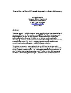
Linear programming is a mathematical technique for optimization of a linear objective function, subjected to linear equality and linear inequality constraints. It can be defined as the problem of maximizing or minimizing a linear function subjected to linear constraints. For example Find numbers x1 and x2 that maximizes x1 + x2 subjected to the constraints x1 ≥ 0, x2 ≥ 0 and x1 + 2x2 ≤ 4

(3.1)

4x1 + 2x2 ≤ 12

(3.2)

−x1 + x2 ≤ 1

(3.3)

This problem contains two unknowns and five constraints. All constraints are inequalities and they are all linear in the sense that each involves an inequality in some linear function of the variables. The first two are called ’nonnegativity’ constraints and are often found in linear programming. The other three constraints are the ’main constraints’. The function to be minimized is known objective function.Here it is x1 + x2 . Since there are only two variables, we can solve this problem by graphing the set of points in the plane that satisfies all the constraints (called the constraint set) and then finding which point of this set maximizes the value of the objective function. Each inequality constraint is satisfied by a half-plane of points, and the constraint set is the intersection of all the half-planes. In the present example, the constraint set is the five-sided figure shaded in figure3.1.

CHAPTER 3. MATHEMATICAL PROGRAMMING

26

We seek the point (x1 , x2 ), that achieves the maximum of x1 +x2 as (x1 , x2 ) ranges over this constraint set. The function x1 + x2 is constant on lines with slope -1, for example the line x1 +x2 = 1, and as we move this line further from the origin up and to the right, the value of x1 +x2 increases. Therefore, we seek the line of slope -1 that is farthest from the origin and still touches the constraint set. This occurs at the intersection of the lines x1 +2x2 = 4 and 4x1 +2x2 = 12, namely,(x1 , x2 ) = (8/3, 2/3) The value of the objective function there is (8/3) + (2/3) = 10/3. All linear programming problems are not so easy solve. There may be many variables which are constrained as nonnegative or unconstrained and many main constraints which are equality or inequality constraints. There are two classes of problems one is the standard maximum problem and the other one is the standard minimum problem. In these standard problems all variables are constrained as non negative and all main constraints are inequality constraints. We are given an m-vector,b = (b1 , ......, bm ), an n-vector, c = (c1 , ...., cn )T , and an m × n matrix, of real numbers   a11 a12 · · · a1n  a21 a22 · · ·    (3.4) A =  .. .. ..  . .  . . . .  am1 am2 · · · amn • The Standard Maximum Problem: Find an n-vector, x = (x1 , ..., xn )T , to maximize cT x = c1 x1 + ... + cn xn (3.5) subjected to the constraints a11 x1 + a12 x2 + .... + a1n xn ≤ b1

(3.6)

a21 x1 + a22 x2 + .... + a2n xn ≤ b2

(3.7)

.. . am1 x1 + am2 x2 + .... + amn xn ≤ bm

(3.8)

Ax ≤ b

(3.9)

x1 ≥ 0, x2 ≥ 0, ...xn ≥ 0

(3.10)

or and

CHAPTER 3. MATHEMATICAL PROGRAMMING

27

or (x ≥ 0)

(3.11)

• The Standard Minimization Problem: Find an m-vector, y = (y1 , ..., yn )T , to maximize y T b = y1 b1 + ... + yn bn (3.12) subjected to the constraints y1 a11 + y2 a21 + .... + ym am1 ≥ c1

(3.13)

y1 a12 + y2 a22 + .... + ym am2 ≥ c2

(3.14)

.. . y1 a1n + y2 a2m + .... + ym anm ≥ cn

(3.15)

y T A ≥ bT

(3.16)

y1 ≥ 0, y2 ≥ 0, ...yn ≥ 0

(3.17)

(y ≥ 0)

(3.18)

or and

or

Note that the main constraints are written as ≤ for the standard maximum problem and ≥ for the standard minimum problem. The introductory example is a standard maximum problem. We now present examples of four general linear programming problems. These are the most extensively studied problem.

3.2.1

Example 1: The diet problem

The problem is defined as supplying the required nutrients at minimum cost. For this problem we consider that n - amount of nutrients required for good health,N1 , ....., Nn m - different types of food that supply the nutrients ,F1 , ....., Fm , cj - the minimum daily requirement of nutrient, Nj bi - the cost for unit of food, Fi aij - the amount of nutrient Nj contained in one unit of food Fi yi - the number of units of food Fi to be purchased per day. To supply the diet

CHAPTER 3. MATHEMATICAL PROGRAMMING

28

that is essential for a day it costs b1 y1 + b2 y2 + ...... + bm ym .

(3.19)

Then the amount of nutrients contain in the provided diet is give by a1j y1 + a2j y2 + ...... + amj ym .

(3.20)

for j = 1, ....., n. The diet is consider to be perfect unless all the minimum daily requirements are met, That means a1j y1 + a2j y2 + ...... + amj ym ≥ cj

(3.21)

for j = 1, ....., n We cannot purchase a negative amount of food, y1 ≥ 0, y2 ≥ 0, ...ym ≥ 0

(3.22)

Our problem is: minimize 3.19subject to 3.21 and 3.22. This is exactly the standard minimum problem.

3.2.2

Example 2: The transportation problem

The problem is to minimize the transportation cost. where I - number of ports supply a certain commodity, or production plants, p1 , ....., PI J - markets to where commodities are shipped,M1 , ....., MJ . Port Pi possesses an amount si of the commodity (i = 1, 2, ...., I), Market Mj must receive the amount rj of the commodity (j = 1, ....., J). bij - the cost of transporting one unit of the commodity from port Pi to market Mj . yij - the quantity of the commodity shipped from port Pj to market Mj . Then transportation cost is give by I X J X

yij bij .

(3.23)

i=1 j=1

The amount of commodity shipped form port Pi is commodity available at port Pi is si We can say J X

PJ

j=1

yij ≤ si f or i = 1, ...., I

yij , and the amount of

(3.24)

j=1

The amount of commodity sent to market Mj is at Mj market is rj , i.e.,

PI

j=1

yij , and the amount required

CHAPTER 3. MATHEMATICAL PROGRAMMING

I X

yij ≤ ri f or j = 1, ...., I

29

(3.25)

i=1

We cannot send a negative amount from PI to Mj , So yij ≥ 0 f or i = 1, ...., I and j = 1, ......, J

(3.26)

Our aim is to minimize 3.23, subjected to 3.24,3.25 and 3.26.

3.2.3

Example 3: The activity analysis problem

This problem is to choose the intensities which the various activities are to be operated to maximize the value of the output to the company subject to the given resources. n - number of activities in a company, A1 , ....An using the available supply of m - number of resources available, R1 , ....Rm (labor hours, steel, etc.). bi - the available supply of resource Ri aij - the amount of resource Ri used in operating activity Aj at unit intensity. cj - the net value to the company of operating activity Aj at unit intensity. xj - the intensity at which Aj is to be operated. The value of such an activity allocation is n X

cj x j .

(3.27)

j=1

The amount of resource Rj used in this activity allocation must be no greater than the supply, bj ; that is, n X

aij xj ≤ bi f or i = 1, ..., m.

(3.28)

j=1

It is assumed that we cannot operate an activity at negative intensity; that is, x1 ≥ 0, x2 ≥ 0, ...., xn ≥ 0.

(3.29)

Our problem is: maximize3.27 subject to 3.28 and 3.29. This is exactly the standard maximum problem.

3.2.4

Example 4 The optimal assignment problem

This is a problem of choosing a person to a job in order to minimize the total cost/value. For this problem we consider I - number of persons available for doing jobs J - number of jobs to be performed

CHAPTER 3. MATHEMATICAL PROGRAMMING

30

aij - cost/value of a person I working on job J per day, where i = 1, ...., I and j = 1, ...., J We have to find an assignment, xij , fori = 1, ...., I and j = 1, ...., J where xij represents the proportion of time person i to spent on job j. Then, J X

xij ≤ 1 f or i = 1, ...., I

(3.30)

xij ≤ 1 f or j = 1, ...., J

(3.31)

j=1 I X i=1

and xij ≥ 0 f or i = 1, ...., I j = 1, ...., J

(3.32)

Our aim is to minimize the total cost/value, I X J X

aij xij .

(3.33)

i=1 j=1

Constraint 3.30 represents that a person cannot work more than 100% of his time,constraint 3.31 means that only one person can work on a job at a time, and constraint 3.32 says that no one can do a negative amount of work. Finally we have to maximize 3.33 subjected to all the constraints 3.30,3.31 and 3.32

3.2.5

Terminology

• The function to be maximized or minimized is called the objective function. • The values of x or y is said to be a feasible solution if it satisfies the constraints. • The set of all feasible values is said to be the constraint set. • A linear programming problem feasible if and only if the constraint set is not empty; otherwise it is infeasible. A linear programming problem may be bounded feasible, unbounded feasible or it may be infeasible.

CHAPTER 3. MATHEMATICAL PROGRAMMING

3.3

31

Quadratic programming

Quadratic programming is a special case of mathematical programming problem with a quadratic objective function to be optimized subjected to a set of linear equality and linear inequality constraints. A quadratic programming problem is formulated as: 1 min f (x) = CX + X T Q X 2

(3.34)

AX ≤ b, X ≥ 0

(3.35)

subjected to

Where C is an n- dimensional row vector describing the coefficients of the linear terms in the objective function and Q is an (n × n) symmetric matrix describing the coefficients of the quadratic terms. The constraints are denoted by (m × n) matrix. A simple numerical example for quadratic programming problem is give as

3.4

min 0.5x21 + 0.1x22

(3.36)

s.t x1 − 0.2x2 ≥ 48

(3.37)

5x1 + x2 ≥ 250

(3.38)

x1 , x2 ∈ R

(3.39)

Production scheduling problem

Most of the production scheduling problems can be modeled as linear programming problems. The linear program can be solved in polynomial time. To show the process of modeling a problem as a linear program we consider a scheduling problem: The three field notation of the problem is give as R|pmtn|Cmax

(3.40)

This represents the the machine environment is a parallel machines which are not related to each other and the job can be preemptive scheduled. The main objective is to minimize the makespane. In order to explain this modeling we use nmvariables xij where 1 ≤ i ≤ m and 1 ≤ j ≤ n . The variable xij denotes the fraction of jobs j that is processed on machine i;for example we would interpret a linear programming solution with x1j = x2j = x3j = 13 as assigning 13 of job j to machine 1, 31 to machine 2 and 13 to machine 3. Now we study the types of constraints to be assigned to job xij so that they describe a valid solution to the problem R|pmtn|Cmax .It is clear

CHAPTER 3. MATHEMATICAL PROGRAMMING

32

that the fraction of job that is processed on a machine xij must be a non negative one. We model this constraint as xij ≥ 0

(3.41)

We can also say that if a job is completely processed than the sum of fraction of job that is processed on a machine must be 1. m X

xij = 1, 1 ≤ j ≤ n

(3.42)

i=1

Our objective is to minimize the makespan Cmax of the schedule. Recall that the amount of processing that job j would require if run entirely on machine i is pij . Therefore for a set of fractional assignments xij we can determine the amount of P time machine i will work: it is just xij pij , which must be at most Cmax . We model this with the m constraints n X

pij xij ≤ D f or i = 1, ....., m

(3.43)

j=1

Finally we must ensure that no job is processed for more than Cmax time. We model this with the n constraints m X

pij xij ≤ D, 1 ≤ i ≤ n

(3.44)

i=1

To minimize, we formulate the problem as the following linear program min Cmax m X

(3.45)

xij = 1, f or j = 1, ....., n

(3.46)

pij xij ≤ D f or i = 1, ....., m

(3.47)

pij xij ≤ D, f or j = 1, ....., n

(3.48)

i=1 n X j=1 m X i=1

xij ≥ 0 f or i = 1, ....., m, i = 1, ....., m

(3.49)

It is clear that any feasible schedule for our problem yields an assignment of values to the xij that satisfies the constraints of our above linear program. But this linear program does not specify the ordering of the jobs on a specific machine but simply assigns the jobs to machines while constraining the maximum load on

CHAPTER 3. MATHEMATICAL PROGRAMMING

33

any machine. In order to specify the order of the jobs we need further modeling of problem. But this will be a Np-hard problem in most of the case. The solution can not be obtained in polynomial time. In the next section we will see some of the relaxations method which resolve a NP-hard problem.

3.4.1

Linear programming relaxation

In order to explain the relaxation methods we consider a linear programming model P which is give by 1|rj , prec| wj Cj .This model is with precedence constrain that means it needs the order of the jobs to be specified. The order of the jobs on a machine is a critical element of high quality solution, so we seek a formulation that can model this problem. We have n variables Cj , one of each job. It represents the completion time of the job in a schedule. The model of this problem is give as X min w j Cj (3.50) j

subjected to Cj ≥ rj + pj , j = 1, 2..., n

(3.51)

Ck ≥ Cj + pk or Cj ≥ Ck + pj f or each pair j, k

(3.52)

Unfortunately the last set of constraints are not linear constraints. We use a class of inequality of constraints instead of these introduced by Queyranne [27]. We denote the entirePset of jobs as NPset of 1, ..., n and for any subset S ⊆ N we define p2 (S) = p2j and p(S) = pj . For any feasible one machine schedule we claim j

j

that X j

1 pj Cj ≥ (p2 (S) + p(S)2 ) 2

(3.53)

Now we show that these inequalities are satisfied by the completion times of any valid scheduling for onePmachine and thus in particular by the completion of a valid schedule for 1|rj , prec| wj Cj Definition: Let C1 , ...., Cn be the completion times of jobs in any feasible schedule on one machine. Then the Cj must satisfy the inequality X j

1 pj Cj ≥ (p2 (S) + p(S)2 ) 2

(3.54)

Proof: We assume that the jobs are indexed so that C1 ≤ .... ≤ Cn . Consider the j P case S = {1, ..., n}Clearly for any job j, Cj ≥ pk . Multiplying by pj and summing k=1

over all j we obtain

CHAPTER 3. MATHEMATICAL PROGRAMMING

n X j=1

p j Cj ≥

n X j=1

pj

34

j X

1 pk = (p2 (S) + p(S)2 ) 2 k=1

It can be applied to any other set of S where we ignore the other jobs. In the case P P of 1|| wj Cj the constraints j pj Cj ≥ 21 (p2 (S) + p(S)2 ) gives an exact characterization of the problem. Specifically any set of Cj that satisfy these constraints must describe the completion times of a feasible schedule. Thus these linear constraints effectively replace Ck ≥ Cj + pk or Cj ≥ Ck + pj f or each pair j, k. Now we no longer have P an exact formulation, but rather a linear programming relaxation of 1|rj , prec| wj Cj . The main goal of the scheduling problem is to find the beginning time of each job so as to minimize the weighted sum of the completion times. We see the solution method of this problem using CNN in the later chapters.

Chapter

4

Lagrangian relaxation 4.1

Introduction

An optimization problem is a problem of finding an optimal solution from a set of feasible solutions. A combinatorial optimization problem is a typical optimization problem where the feasible solutions can be reduced to discrete set. Generally combinatorial optimization problems are of two categories: one is ’easy’ and the other one is ’hard’ [28]. The optimization problems that are said to be easy can be solved in real time i.e., polynomial time, while the optimization of hard problems cannot be done in polynomial time. These are known as NP hard problems. There are some pseudo-polynomial algorithms available to solve ’easier hard’ optimization problems in polynomial time. In the early 1970s the optimization problem is represented with an simple objective function subjected to complex constraints. These constraints make the problem hard. In order to solve these hard problems the constraints are relaxed using some relaxation methods. There are so many relaxation methods in use to make a hard problem simple. In the next sections we will see how relaxation is done and what are the properties the relaxed problem must have and how to evaluate the quality of problem.

Notation If P is an optimization problem, the notation used for it is F S(P ), the of feasible solutions of problem P OS(P ), the set of feasible solutions of problem P v(P ), the set of optimal solution of problem P

35

CHAPTER 4. LAGRANGIAN RELAXATION

4.2 4.2.1

36

Relaxation method Relaxation of optimization problem

The relaxation of a minimization problem is formally defined as follows [29] Definition: Problem (RPmin ):min{g(x)|x ∈ W } is a relaxation of problem (Pmin ): min{f (x)|x ∈ V }, with the same decision variable x, if and only if 1. The feasible set of (RPmin )contains that of (Pmin ), i.e., W ⊇ V , and 2. Over the feasible set of (Pmin ), the objective function of (RPmin )dominates (is better than) that of (Pmin ), i.e., ∀x ∈ V , g(x) ≤ f (x). If the original problem is a maximization problem then the definition will be Definition: Problem (RPmax ):max{g(x)|x ∈ W } is a relaxation of problem (Pmax ): max{f (x)|x ∈ V }, with the same decision variable x, if and only if 1. The feasible set of (RPmax )contains that of (Pmax ), i.e., W ⊇ V , and 2. over the feasible set of (Pmax ), the objective function of (RPmax )dominates (is better than) that of (Pmax ), i.e., ∀x ∈ V , g(x) ≥ f (x). It follows that for the minimization problem v(RPmin ) ≤ v(Pmin ) and for maximization problem v(RPmax ) ≥ v(Pmax ), in both cases we can say that (RPmin )is an optimistic version of (Pmin ). The results in both the cases can be easily translated from one type to the other by remembering that max {f (x)|x ∈ V } = − min {−f (x)|x ∈ V }

(4.1)

The relaxation method provides bounds on the optimal value of difficult problem, and the solution obtained can also be used as a starting point for the specialized heuristics.

4.2.2

Lagrangian relaxation

Lagrangian relaxation is a relaxation technique widely used for the linear programming problems [29]. we will see some characteristics of Lagrangian relaxation method. Let P is a optimization problem of the form min {f (x)| Ax ≤ b, Cx ≤ d, x ∈ X}

(4.2)

where X may contain non-negative integers or any other set which restricts the solution set of the optimization problem. The constraint Ax ≤ b is assumed to be a

CHAPTER 4. LAGRANGIAN RELAXATION

37

complicated one. Then the Lagrangian relaxation of P can be given by relaxing the complicated constraint keeping the other constraints unmoved. The Lagrangian relaxation of P relative to the complicating constraint Ax ≤ b, with non-negative Lagrangian multiplier λ, is as follows min {f (x) + λ(Ax ≤ b)| Cx ≤ d, x ∈ X}

(4.3)

Here the complicated constraint Ax ≤ b is added to the objective function with weight λ and is released from the constraint list. This is known as dualized problem. The problem is relaxation of P since for any x feasible for P and for λ ≥ 0, f (x) + λ(Ax ≤ b) is less than or equal to f (x).

4.3

Example

We now see the application of Lagrangian relaxation method to an integer problem. This problem is a generalized assignment problem [30, 31]. Z = min

n m X X

Cij xij

(4.4)

i=1 j=1 m X

xij = 1, j = 1 , ....., n.

(4.5)

aij xij ≤ bi , i = 1 , ......, m

(4.6)

i=1 m X j=1

xij = 0 or 1, all i and j

(4.7)

The natural Lagrangian relaxation for this generalized assignment problem can be obtained in two ways: by relaxing the constraints (4.5) or (4.6). The dual problem obtained by dualizing the constraint (4.5) is ZD1 = min

m X n X

Cij xij +

i=1 j=1

n X

λj (

m X

j=1

xij − 1)

(4.8)

i=1

subjected to m X

aij xij ≤ bi , i = 1 , ......, m

(4.9)

j=1

xij = 0 or 1, all i and j We can rewrite the above dual problem as

(4.10)

CHAPTER 4. LAGRANGIAN RELAXATION

ZD1

38

n X m n X X = min (Cij + λj )xij − λj i=1 j=1

(4.11)

j=1

subjected to m X

aij xij ≤ bi , i = 1 , ......, m

(4.12)

j=1

xij = 0 or 1, all i and j

(4.13) m P

This problem can be solved in time proportional to n

bi as it resembles the knap-

i=1

sack problem.Another dual problem is obtained by dualizing constraint (4.6) is ZD2 = min

m X n X

Cij xij +

i=1 j=1

n X i=1

n X aij xij − bi ) λj (

(4.14)

j=1

subjected to m X

xij = 1, j = 1 , ....., n.

(4.15)

i=1

xij = 0 or 1, all i and j

ZD2 = min

n m X X i=1

(4.16)

! (Cij + λi aij )xij

j=1

−

m X

λi bi

(4.17)

i=1

subjected to m X

xij = 1, j = 1 , ....., n.

(4.18)

i=1

xij = 0 or 1, all i and j

(4.19)

Now we can observe that the relaxed assignment problem equation (4.17) is a simple multiple choice problem. For both the dual problems λ ≥ 0, which is necessary condition for ZD ≤ Z.

4.4

Lagrangian relaxation neural networks

The Lagrangian relaxation neural networks (LRNN), which deals with the dynamics of neurons, is a combination of recurrent neural network optimization idea with Lagrangian relaxation for constraint handling. This method is better explained with an example. To understand the basic idea behind this approach clearly we consider a separable convex programming problem [31].

CHAPTER 4. LAGRANGIAN RELAXATION

39

Let J is a separable convex programming problem min J ≡ x

I X

Ji (xi )

(4.20)

i=1

subjected to I X

gi (xi ) ≤ 0 i = 1, ...., I

(4.21)

i=1

where xi ∈ RNi is a Ni ×1 continuous decision variable with

I P

Ni = N , {Ji (xi )} and

i=1

{gi (xi )} are convex and differentiable functions, and I is number of sub-problems. Since both objective function and constraint function are additive, the problem is separable.First we apply Lagrangian relaxation for this minimization problem. As explained earlier it is just moving the constraint function gi (xi ) ≤ 0 into the objective function with a non-negative weight, Lagrangian multiplier λ " L(λ) ≡ min

I X

x

Ji (xi ) + λT

i=1

I X

# gi (xi )

(4.22)

i=1

The function L(λ) is known as Lagrangian dual (LD) function. As the decision variables are decoupled through the relaxation method, the equation can be written as sub-problems: " I # I X X Li (λ) ≡ min Ji (xi ) + λT gi (xi ) , (4.23) xi

i=1

and L(λ) =

i=1 I X

Li (λ)

(4.24)

i=1

The dual problem is then given by LD : max L(λ) λ≥0

(4.25)

The dual function is always a convex function. The main idea behind Lagrangian relaxation neural networks is to create a network and let the negative dual be its energy function. The negative dual will naturally approaches to its minimum, as the network converges and then x? , a minimum solution, can be found  I easily. TheI negative  dual is taken from the relaxed funcP P tion Li (λ) ≡ min Ji (xi ) + λT gi (xi ) or from the sub-problem Li (λ) . The xi

i=1

i=1

CHAPTER 4. LAGRANGIAN RELAXATION

40

relaxed problem which is free of constraints can be solved using recurrent neural network. Finally the main idea behind the Lagrangian relaxation neural network is to merge these two constructs, one for the negative dual and the other for the relaxed problem, and let them feed each other and converge simultaneously. The network elements that updates the multiplier and solve sub-problem are known as Lagrangian neurons and decision neurons respectively. The dynamics of Lagrangian relaxation neural networks is described by the following equations

dλm (t) = dt

( 0

f or λm (t) = 0 and

˜ α(t) ∂ L(λ(t),x(t)) ∂λm (t)

˜ ∂ L(λ(t),x(t)) ∂λm (t)