A Brief Introduction to Fitting Models and Parameter Estimation Least Squares Fitting Suppose we have N pairs of observations, (x1 , y1 ), . . . (xN , yN ) and we expect x and y to be related according to some function, g, which itself involves one or more parameters, which we write as the vector a. y = g(x; a). Typically, the points (xi , yi ) won’t fall exactly on the curve. (Why? We might have measurement error or perhaps the relationship doesn’t exactly follow the function given). We need to find the value of the parameter vector a that makes the function g(x; a) provide the best fit to the data points. One measure of how well the data fits is to take the difference between the predicted value of y and the observed value of y (we call this the error), square it (to get the squared error), and add up all these quantities for each of the data points (the sum of squared errors, or the error sum of squares, often abbreviated as the sum of squares). 0.8
0.6
(x2,y2)
y
e1
e2
0.4
(x3,y3) e3
(x1,y1) 0.2
e4 (x4,y4)
0
1
2
x
3
4
(Why don’t we just work with the unsquared errors? Positive and negative differences can cancel. Why not the absolute values of the errors? It turns out the math is easier.) For our data point (xi , yi ), the predicted value of y is g(xi ; a) so our sum of squares is
L(a) =
N X
(yi − g(xi ; a))2 .
i=1
Obviously, the sum of squares depends on the parameter vector a, so we write L as a function of a. Our task is now to find the minimum of L(a) over different values of a. In general, this is not a straightforward task. If the function g is linear in its parameters then we can make analytic progress. One example of this is simple linear regression.
Linear Regression Suppose we have N pairs of observations, (x1 , y1 ), . . . (xN , yN ) and we expect x and y to be linearly related: y = ax + b. We want to minimize the sum of squares
L(a, b) =
N X
(yi − (axi + b))2 ,
i=1
over the parameters a and b. This is a simple problem, often seen in multivariable calculus courses. We solve ∂L =0 ∂a
∂L = 0. ∂b
and
Let’s first look at ∂L/∂b. ∂L ∂b
N X
=
2(−1) (yi − (axi + b))
i=1
= −2 = −2
N X
(yi − axi − b)
i=1 N X
= −2
i=1 N X
N X
yi − a
i=1 N X
yi − a
i=1
xi −
N X
!
b
i=1
!
xi − bN .
i=1
Setting the partial derivative equal to zero we get 0 = ⇒ ⇒
1 N
N X i=1 N X
N X
yi − a
i=1 N X
yi = a yi =
i=1
xi − bN
i=1
xi + bN
i=1 N X
a N
N X
(1)
xi + b
i=1
⇒ y = ax + b.
(2)
Here, y denotes the average of the yi and x denotes the average of the xi . We see that the best fitting straight line passes through the “average” of the data points, (x, y). Looking at the other partial derivative: ∂L ∂a
=
N X i=1
−2xi (yi − (axi + b))
= −2 = −2
N � X
xi yi − ax2i − bxi
i=1 N X
xi yi − a
N X
x2i
�
−b
!
xi .
i=1
i=1
i=1
N X
Setting the partial derivative equal to zero gives N X
1 N
i=1 N X
xi yi = a
N X
x2i + b
i=1 N X
a N
xi yi =
i=1
⇒ xy =
xi
(3)
i=1
x2i +
i=1
ax2
N X
N b X xi N i=1
+ bx.
(4)
Here, xy means the average value of xi yi and x2 is the average value of x2i . Notice that in general, xy 6= x · y and x2 6= (x)2 . Equations (1) and (3) (or the pair 2 and 4) are a pair of simultaneous linear equations for a and b and can be written as the matrix equation
P x P 2i
xi
N P xi
!
a b
!
=
P y P i
xi yi
!
.
In this form, the equations are usually referred to as the normal equations. (Here, all sums are taken from i = 1 to i = N .) Provided that the matrix on the left hand side is invertible, these are easily solved for a and b. Equivalently, we can work with equations 2 and 4 and get x 1 x2 x
!
a b
!
=
y xy
!
.
These are just the normal equations divided by N . Either set can be solved to give a =
xy − x · y x2 − x2
x2 · y − x · xy x2 − x2 = y − ax.
b =
Thinking back to our problem of minimizing L(a, b), we should also check that the point we get is a minimum (how do you do this?). We now have our best fitting straight line.
*More General Linear Regression (A starred section is one that you would not be expected to know the details of for the test.) It turns out that we can apply this procedure to fit a general linear model of the form yi =
k X
bj gj (xi ) + ei ,
j=1
where the bj are constants and the gj are any functions (not necessarily linear) of x alone. By “linear” here we mean that the model is linear in the parameters bj , not (necessarily) in x. We write the number of parameters as k. Our linear regression model can be written in this form by taking b1 = b, b2 = a, g1 (x) = 1, g2 (x) = x. We could fit a quadratic model by adding b3 = c and g3 (x) = x2 , giving y = b + ax + cx2 . The solution for the “best fitting” set of parameters bi is usually obtained via a matrix calculation. Various similar quantities are grouped together into matrices and vectors. The N observations get stacked up in the vector y and the k parameters in the vector b. The (i, j) entry of the N × k matrix X is set equal to gj (xi ). This allows the model to be written as y = Xb + e, where e is a vector containing the N “errors”. As in the linear regression analysis, we can find the best fitting value of b, often written as ˆ by calculating the partial derivatives of the function L(b) with respect to each of the bj , b setting the derivatives equal to 0 and solving. It turns out that this gives the following set of normal equations ˆ = X T y. X TX b Notice that the normal equations are linear for the general linear model. If the matrix X T X is invertible, the normal equations can be solved to give �
ˆ = XT X b The matrix X T X has (i, j) entry equal to P equal to k gi (xk )yk .
�−1
P
X T y.
k gi (xk )gj (xk )
and the matrix X T y has entries
Fitting Different Models (not starred!) Imagine fitting the straight line y = a + bx and the quadratic y = a + bx + cx2 to the same set of data. Which would fit better? (In other words, have a smaller minimum sum of squares?) The quadratic must fit better. Why is that? Because the straight line is a special case of the quadratic (with c = 0), so the best fitting quadratic can never do any worse than the best fitting line. The quadratic is more flexible in this sense. This is a general point: if we have a more flexible function, we will be better able to fit data. If we took higher and higher degree polynomials, we could improve further. (A polynomial of degree n means that there will be n + 1 simultaneous linear equations to solve.) We can find a straight line that perfectly fits a data set consisting of any two points (unless they lie on a vertical line). We can find a quadratic equation that perfectly fits (almost any) data set consisting of three points. And so on... By making our function sufficiently complex we can often make it pass through all of the points, even though the data contains error (e.g. measurement error). The point is that complex functions are prone to overfitting data. (Remember the point about us preferring simple models over complex ones?) Statisticians have a methodology to answer the following questions raised by these considerations: • Does one model fit “significantly” better than another? • Does the improved fit justify the additional complexity of the model?
Nonlinear Least Squares: Moving Beyond Linear Models What happens if we try to fit an exponential function directly to the population growth data? (Earlier on we talked about converting the exponential growth of the population data to linear growth by logging the data.) To simplify, let’s just fit the model y = eax to some data. (Imagine we can set the initial value equal to one.) Then we have L(a)
=
X
(yi − eaxi )2
∂L ∂a
=
−2
X
=
−2
�X
⇒
xi eaxi (yi − eaxi ) xi yi eaxi −
X
�
xi e2axi .
X X ∂L =0 ⇒ xi yi eaxi = xi e2axi . ∂a
Can we solve for a? Looks unlikely: the normal equations are nonlinear, with a appearing in the exponent of a sum of (up to) 2N exponential terms.
The key difference is that a polynomial is linear in its parameters, the exponential is nonlinear in its parameter. This leads to the normal equations being linear (easy to solve) or nonlinear (difficult to solve), respectively. For a nonlinear model we typically cannot solve the least squares problem analytically. Instead we turn to numerical approaches. Numerical optimization is, in general, a non-trivial problem. Finding a minimum is easy if a function has a single minimum— you just vary the parameter value so that you move “downhill” towards the minimum. More generally, functions have one or more local minima in addition to their global minimum. It is then not easy for an optimization routine to figure out whether a minimum is just a local one or is the global minimum. 10
20 15
6
L(a)
L(a)
8
4
5
2 0
10
0
1
2
a
3
4
5
0
0
1
2
a
3
4
5
Figure 1: The minimum of the function in the left hand panel is easily found, but the local minima in the right hand panel make the process more difficult.
People spend their entire careers working on minimization problems, but this isn’t a course on numerical analysis and optimization. We will follow the many people who typically (and often over-optimistically) don’t spend too much time worrying about this. Usually, they employ a pre-packaged optimization routine and hope that everything will be OK. MATLAB provides several such routines, and fminsearch seems to be a popular choice. We will soon discuss using MATLAB to fit population growth models. Other points: • Finding a minimum may become more difficult if our model has more parameters since we have a larger “parameter space” to explore. • What does the shape of L(b) near its minimum tell us about how accurately we can find the values of parameters?