TSTE80 ATIK and TSEI30 ANTIK

7

Lecture 7 — Operational Amplifiers II

Operational Amplifiers II Part 7.A—Repetition Single-pole and dual-pole systems General approximation of a multi-pole system:

A0 A(s) = --------------------------------------------s  s  1 + ----⋅ 1 + -----  p 1  p q Zeros and poles are approximated by an equivalent pole p q . If we have a second pole dominating over other higher poles, p q ≈ p 2 ( p q > p 2 ) . A two-pole system in a feedback loop

β2 X(s)

Figure 7.1:

a(s)

Y(s)

Amplifier with feedback.

“Optimal” behavior (bandwidth usage) for Q = 1 ⁄ 2 gives a phase margin ϕ m ≈ 67° . Design goal should be in the order of 75 degrees in order to have a proper design margin. Design requirements put on the phase margin, the equivalent pole, and the Q -value. The Q -value is also given by the feedback factor β :

β ⋅ A0 ⋅ p1 Q ∼ ----------------------pq Passive compensation Introduce a capacitance C c between the output of the stages. We have that the first pole now ends up at

g I ⋅ g II p 1 ≈ --------------------g mII ⋅ C c Hence the pole is moved down and this is referred to as the Miller effect. Sometimes we refer to this kind of capacitance as the Miller capacitance. We also have that the second pole is linearly dependent on the g mII , and

1 p 1 ∼ ---------- and p 2 ∼ g mII g mII This is referred to as pole splitting.

Department of Electrical Engineering, Linköpings universitet

83

84

TSEI30 ANTIK and TSTE80 ATIK

Department of Electrical Engineering, Linköpings universitet

Basically: How can we achieve high p 1 , high A 0 at the same time as p 2 ( p q ) is much more higher (improved phase margin)?

If a low output impedance is needed, the output current may be increased in order to reduce the output impedance or a there is a need for an additional source-follower at the output to lower the output impedance.

Basically if we are driving capacitive loads only, OTAs and OPs can be used. Therefore, we can increased the output impedance in order to increase the gain for high accuracy applications.

The difference between the Gm and the OTA is given by the fact that the Gm should have a fixed transconductance value over a large input voltage range. Therefore linearization circuits are mostly needed.

The difference between the OTA and the OP is given by the fact that the operational amplifer should have a zero output impedance whereas the OTA should have an infinite output impedance.

Part 7.B—High-performance operational amplifiers

The latter is referred to as pole-zero cancelling.

1 1 R c = ---------- or R c = --------------------- ⋅ ( C I + C II + C c ) g mII ⋅ C c g mII

The zero can now be cancelled by either letting it move towards infinity or to cancel the second pole p 2 . This calls for two different options:

1 R c + --------sC c

The Miller compensation introduces a zero in the RHP which destroys the phase. This can be removed by adding a resistance in series with the capacitance:

High-performance operational amplifiers

M3

M1

M2

M4

Comp.

Vin+

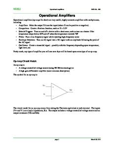
A two-stage OP/OTA with compensation circuit.

Ibias

Vin-

M5

M7

CL

Vout

Department of Electrical Engineering, Linköpings universitet

• Poorly separated poles (compensation often required).

• Low-voltage operation.

• Controlled DC voltages (equal input and output voltages possible)

85

• Insensitive to load capacitance due to the compensation capacitance and the pole splitting.

• Distribute the gain in the two stages so that the Miller effect and p 2 are controlled.

Design issues • Systematic offset

(We only consider Miller compensation). We find that we can increase the p 2 by increasing g mII . If we increase the area of the transistor ( W ) the capacitance C I will however increase even faster and then the p 2 will in fact decrease.

I6   I5 SR = min  ------------------, --------------------   C c + C I C c + C II 

g mI ω u = ------Cc

1 z = -------------------g mII ⁄ C c

2 g mII g mII C c g ds - and p 2 = ------------------------------------------------------ ≈ -------------------p 1 = -------------------C c C I + C c C II + C I C II C I + C II g mII ⋅ C c

The output from the first stage is connected to a high-impedance node at the input of the first stage (high R and high C). Therefore, the poles are poorly separated.

Figure 7.2:

M8

M6

Lecture 7 — Operational Amplifiers II

Consider the compensated two-stage amplifier in the figure.

Part 7.C—Two-stage amplifier

TSTE80 ATIK and TSEI30 ANTIK

86

A telescopic-cascode OTA.

Ibias

Vin+

M4

M3

Vout

M7

M10

M2

M9

M8

M1

M5

Vin-

TSEI30 ANTIK and TSTE80 ATIK

• Well separated poles

• High-voltage operation

Department of Electrical Engineering, Linköpings universitet

• Equal input and output DC voltages not feasible

• Sensitive to load capacitance

Design issues • Gain in one stage only – simpler design

I5 SR = -----CL

g m1 ω u = -------CL

2 2 ⋅ g ds g m7 p 1 = --------------- and p 2 = -------------------------------------------g m7 C L C gs7 + C gd1 + C b7

One-stage amplifier with low impedance nodes. High output impedance in order to increase DC gain and the poles become well-separated poles

Figure 7.3:

M6

Part 7.D—Telescopic-cascode amplifier

Telescopic-cascode amplifier

M10

M8

M6

Vin-

A folded-cascode amplifier.

Vbias2

Vbias1

M3

M1

M5

M2

Vin+

M9

M7

Vbias1

M11

Vbias2

M4

CL

Vout

Lecture 7 — Operational Amplifiers II

Department of Electrical Engineering, Linköpings universitet

5 I 4 = 5 ⋅ I 7 = --- I 5 . 8

• Choose I 1 ≈ 4 ⋅ I 7 . We have I 5 = 2 ⋅ I 1 and I 4 = I 1 + I 7 , which gives that

• Well separated poles due to high output impedance

• Low-voltage operation possible

• Controlled DC voltages (equal input and output voltages possible)

Design issues • Sensitive to load capacitance

I4 SR = -----CL

gm ω u = -----CL

2 g ds g m7 p 1 = ------------ and p 2 = -------------------------------------------------------------gm C L C gs7 + C gd4 + C gd4 + C b7

87

One-stage amplifier with internal low impedance nodes. High output impedance in order to increase DC gain and the poles become well-separated poles

Figure 7.4:

M13

Ibias2

Ibias1

M12

Part 7.E—Folded-cascode amplifier

TSTE80 ATIK and TSEI30 ANTIK

88

Vin-

M1

Vbias0

A current-mirror amplifier.

M12

M10

M8

M3

M5

M2

M9

M4

Vin+ M13

M11

CL

Vout

Vbias2 M15

M7

TSEI30 ANTIK and TSTE80 ATIK

Department of Electrical Engineering, Linköpings universitet

• I 1 ≈ 4 ⋅ I 7 gives that I 4 = I 1 + I 7 = 5 ⋅ I 7 . I 5 = 2 ⋅ I 1 . I 4 = 2.5 ⋅ I 5 .

• Well separated poles due to high output impedance

• Low-voltage operation possible

• Controlled DC voltages (equal input and output voltages possible)

Design issues • Sensitive to load capacitance

K⋅I SR = ------------5CL

K ⋅ g m1 ω u = ----------------CL

g m4 p 1 = ------------- and p 2 = ------------------------------------------------------------------------------------------------gm C L C gs4 + C gs7 + C gd6 + C gd8 + C gs9 + C b4

2 g ds

One-stage amplifier with internal low impedance nodes. High output impedance in order to increase DC gain and the poles become well-separated poles

Figure 7.5:

M14

Vbias2

Vbias1

M6

Part 7.F—Current-mirror amplifier

Current-mirror amplifier

Lecture 7 — Operational Amplifiers II

Differential operational amplifier.

Vout

Vin-

Vin+

=

x

x

A d A cm

⋅

∆V out ∇V out

Department of Electrical Engineering, Linköpings universitet

89

Poor gain of the common-mode signal in the feedback loop and therefore we need a special feedback circuit in order to achieve high common-mode gain and hence stabilize the common-mode voltages.

Common-mode feedback circuit, CMFB

We consider the differential gain and the common-mode gain.

∇V out

∆V out

The output voltages (or the transfer function) are given by

+ + V+ + VV in V out in out - and ∇V out = --------------------------∇V in = ---------------------2 2

The common-mode input and ouptut voltages are given by

+ – V - and ∆V + ∆V in = V in in out = V out – V out

Vout+

Vout-

Fully Differential

The differential input and output voltages are given by

gure 7.6:

Vin-

Vin+

Single-Ended Output

Hence only the odd terms are left and even terms are eliminated. Therefore, using differential signals, we have a gain in performance (linearity).

3 +… V out, diff = 2a ⋅ V in + 2c ⋅ V in

+ = – V - = V , we have If we assume that the input signals are perfect, hence V in in in that

+ – V+ + 2 - 2 V out, diff = V out out = a ⋅ ( V in – V in ) + b ⋅ ( ( V in ) – ( V in ) ) + …

The difference between the output signals is

- + b ⋅ ( V - )2 + c ⋅ ( V - )3 + d ⋅ ( V - )4 + … = a ⋅ V in V out in in in

+ + + b ⋅ ( V + ) 2 + c ⋅ ( V + ) 3 + d ⋅ ( V + ) 4 + … and = a ⋅ V in V out in in in

Again assume that we have a positive and negative input through this system (consider the AC signals):

2 + c ⋅ V3 + d ⋅ V4 + … V out = a ⋅ V in + b ⋅ V in in in

Assume that we have a non-linear transfer function

Part 7.G—Fully-differential amplifers

TSTE80 ATIK and TSEI30 ANTIK

90

TSEI30 ANTIK and TSTE80 ATIK

gure 7.7:

Department of Electrical Engineering, Linköpings universitet

Continuous-time CMFB circuits.

Examples (see Johns&Martin for illustrative examples):

The input voltages of the CMFB are the positive and negative output voltages from the differential amplifier. We have that the output voltage (or current) should be a function of the common-mode signal and not a function of the differential signal.

Fully-differential amplifers