5. Fiscal statistics for Sweden, 1670–2011* Klas Fregert and Roger Gustafsson

5.1. Introduction This chapter presents data on central government fiscal measures in Sweden, starting in 1670. Annual data on central government debt are presented from 1670, and on expenditures and revenues from 1719. The aim is to construct measures that are broad, meaningful, and widely used. In practice, this means constructing measures according to the principles in Sweden’s current budget system. Sweden is well suited for this attempt. First, it has been territorially and politically stable to an unusual degree since 1719, when a new instrument of government (regeringsform) was adopted with a representative government. Second, annual data are available in printed form for the whole period. We use Simonsson (1918) for the data on debt in 1670–1718. For the period 1719–1809 we use Åmark’s (1961) monumental study based on archival material. For the period 1810-20 we use Rathsman (1855). From 1821 onwards we use government publications.1 The sources are listed in “Data sources” at the end of the chapter. The chapter is organized as follows. Section 2 presents the definitions used in the calculations. Section 3 describes the flow variables (expenditures, revenues and deficits), section 4 the construction and evolution of debt for the fiscal branch of the central government. Section 5 presents consolidated measures for the fiscal and monetary branches of the central government, including seigniorage. Section 6 concludes. A companion working paper, Fregert and Gustafsson (2005), describes the data in more detail in a series of appendices, as well as the institutional setting. The connections between Sweden’s fiscal and monetary histories from 1668 to 1931 are analysed in Fregert and Jonung (1996).

*

The chapter is an update of Fregert and Gustafsson (2008). 1 International data on government debt are tabulated in Reinhart and Rogoff (2009, appendix A.2).

184

Historical Monetary and Financial Statistics for Sweden, Volume II

5.2. Definitions2 5.2.1. The territory Swedish territory has been constant since 1809. From the mid-1600s, the Swedish state ruled over Estonia, Livonia and Ingria, Pomerania, Wismar and Finland.3 Estonia, Livonia and Ingria were lost in 1721, i.e. before our series of expenditures and revenues start. Separate budgets for Pomerania and Wismar were drawn up by their administrations and had to be approved by the Swedish Parliament. Occasionally, funds were transferred from Sweden to Pomerania, but not the other way. These expenditures appear in the Swedish budgets as “payment to fill the state deficit in Pomerania”. Separate budgets for Finland were drawn up in Sweden from 1722 to 1792; however, as we cannot distinguish Sweden from Finland in the period 1793– 1809, Finland is included in the figures for 1722–1809.4 Furthermore, the year 1809 also represents a break in the data sources. From 1815 to 1905 Sweden was in a union with Norway with the Swedish king as head of state; each country had its own administration and budget but foreign policy was run by Sweden and the cost of the Swedish Ministry of Foreign Affairs was shared.

5.2.2. The central government The central government is a part of general government, which in turn is a part of the public sector, as outlined in Figure 5.1 in accordance with the UN System of National Accounts (SNA) 2008. The defining characteristic of the central government relative to public corporations and social security is that it is financed mainly by taxes. A practical definition of the central government is the activities that appear in current official budgets. Thus, we do not include either public corporations, such as the national railway system and the social security system, or local and regional government. However, the public corporations’ net revenues are included because they are owned by the central government. In official government accounts, the central bank is treated like any other public corporation, such that only its transfers to the treasury enter the budget and borrow2 See Blejer and Cheasty (1991) for a general discussion of definitions and measurement problems. 3 Finland was ceded to Russia in 1809 after a war. Pomerania was occupied by France in 1807 and ceded formally in 1815. Wismar was “lent” to Mecklenburg in 1803 against a down payment to Sweden; Sweden had the right to repurchase Wismar after 100 years at the price of the down payment compounded at 3 per cent annual interest; in reality this was a sale, since neither party foresaw a return to Sweden. 4 The size of the Finnish budget varied over the years but was usually less than 10 per cent of the total budget; the annual average in 1722-92 was 8.2%. Incomes and expenditures are given separately for Finland and Sweden in Åmark (1961, Table 1, pp. 130-141).

Fiscal statistics for Sweden 1670–2010

185

ing at the central bank is lumped together with other borrowing. This concept of the central government may be labelled the central government’s fiscal branch. Since the central bank has a special position as a source of finance for the central government’s fiscal branch, for some macroeconomic purposes it may be preferable to consolidate the central government’s monetary and fiscal branches, which we do in section 6. Figure 5.1. The public sector

Local and regional government

Much of the practical work is done on the consolidation of entities that today constitute the central government’s fiscal branch but earlier were separated institutionally and therefore had separate “off-budget” accounts. Figure 5.1 and Table 5.1 give an overview of how revenues and expenditures have been consolidated. The central government proper (Statsverket), with its own budget and accounts, has always been a subset of our concept the central government. The official budget has been consolidated gradually. The split was largest before 1809, when a number of special funds existed (see Table 5.2). The special funds and the National Debt Office had their separate budgets and earmarked revenues. In 1809, the special funds disappeared as separate agencies, and the National Debt Office’s accounts were included in the official budget. An ancient agency, the National Board of Trade (Kommerskollegium), had previously been financed within the budget but appeared off budget from 1809 to 1874.5 It has been included, though the numbers are insignificant. After 1809, the only major item outside the budget has been government lending to public corporations for investment purposes and later also to private companies (private railways) and individuals (mortgage lending and student loans). Most of the lending was undertaken by the National Debt Office, though the government proper occasionally also lent some means. The traditional term for this lending has been net lending.6 In 1912–1937 and from 1997, net lending was included in the budget. For the periods 1854–1911 and 1938/39–1995/96 we add net lending to the expenditure side. 5 From 1809, Konvojfonden and Krigsmanhuskassorna were included in the government proper (Statsverket), while Manufakturfonden was administered by the National Board of Trade. 6 This is the term used in Blejer and Cheasty (1991), see also below on the definition of the deficit.

186

Historical Monetary and Financial Statistics for Sweden, Volume II

Table 5.1. Consolidation of the central government 1722–2003 Years 1722–1766 1766–1788 1789–1809 1810–1853 1854–1911

Revenues GP + NDO + SF GP + SF GP + NDO + SF GP + SF GP + SF (1854 – 1873)

Expenditures GP + NDO + SF GP + SF GP + NDO + SF GP + SF GP + SF (1854 – 1873) + NL (1854 – 1911) 1912–2011 GP GP + NL (1938/39 – 1995/96) Note: GP = Government proper, NDO = National Debt Office, SF = Special Funds, NL = Net lending.

Table 5.2. Special funds. Name in Swedish Generalförrådskassan Krigsmanshuskassorna Konvojfonden

Landhjälpsfonden

Manufakturfonden Manufakturdiskontfonden Slottsbyggnadsfonden Kommerskollegium Source: Åmark (1961).

Maximum revenue, dsm (year) Funding of temporary 1721–1775 114,795 military needs (1766) Pension fund for retired 1722–1809 109,284 military (1809) Military convoys to escort 1726–1809 440,550 (1778) Swedish ships, financed by export and import duties 1727–1739 Subsidized lending to manufacturing, financed by import duties Successor to 1739–1766 373,346 Landhjälpsfonden (1750) Lending agency for 1756–1776 manufacturers Tax financing of the new 1728–1777 114,828 royal castle in Stockholm (1756) National Board of Trade 1809–1874 Explanation

Years

Maximum debt, dsm (year) 46,887 (1740) 74,982 (1729) 2,107,253 (1776)

3,380,381 (1757)

5.2.3. Government accounts and deficit measures Until 1980 the government accounts have been presented in the form of financial statements divided into two equal-value columns of sources and uses of funds. This corresponds to the one-period central government budget constraint, which shows sources of funds as being equal to uses: Tt + CBTt + Lt = Gt + It + itBt–1 + DAt + AMt . Sources

Uses

(1)

Fiscal statistics for Sweden 1670–2010

187

The sources of funds consist of: Tt the government’s revenues from taxes, income from public corporations and sales of real assets (privatizations), CBTt revenue transfers from the central bank, and Lt new loans. Uses of funds consist of: Gt current expenditures (consumption and transfer payments), It real investments and longterm financial investments (net lending), it Bt–1 nominal interest payments on government debt Bt, DAt changes in short-term financial assets, and AMt amortization of debt (buy-backs and principal payments). The change in government debt in turn is equal to new loans, Lt, minus amortization of government debt, AMt, so (1) may be written: Tt + CBTt + DBt = Gt + It + itBt–1 + DAt . Sources

(2)

Uses

We calculate the total budget deficit as total expenditures minus total revenues, also commonly labelled the government’s borrowing requirement. Rearranging (1) and (2) gives the link between the total deficit and its financing:7 DEFt = (Gt + It + itBt–1) – (Tt + CBTt ) = Lt – AMt – DAt= DBt – DAt . (3) A positive deficit is thus financed by increasing government debt or by selling financial assets.8 An increase in debt that exceeds required borrowing, DEFt, leads to an increase in short-term financial assets, DAt. If the government is running a surplus, it amortizes debt or accumulates financial assets. Changes in financial assets arise naturally from the uneven timing of revenues, expenditures and borrowing operations. They can also arise from the planned delay of expenditures from one year to the next as some revenues are allocated for use over more than one fiscal year. These means are then carried across years as “unspent balances” or “reservations”. The change in short-term financial assets is usually small and consists mostly of changes in the National Debt Office’s and the central government proper’s checking accounts at the central bank. The source-use account statement is presented in Table 5.3. Identifying the deficit involves separating revenues and expenditures, on the one hand, from financing operations, on the other. By convention, expenditures and revenues, the left-hand side of equation (3), are said to appear “above the line”, and financing operations, the right-hand side, appear “below the line”, where the line is the total deficit line drawn in Table 5.3. 7 This is not a true accounting identity, since it leaves out changes in debts and assets unrelated to transactions. With real data accounting errors must also be added. 8 Financing by high-powered money does not appear explicitly as all new debt, whether sold to the public or the central bank, is included for the fiscal branch (the official budget). When the fiscal and monetary branches are consolidated, high-powered money appears explicitly as shown in section 5.

188

Historical Monetary and Financial Statistics for Sweden, Volume II

Table 5.3. The government budget and the total deficit line Sources Uses Net: Uses– sources Revenues: taxes, sales of real Current expenditure, Gt assets, income from public corporations, Tt Transfers from the central Investment, It bank, CBTt Interest payments, it Bt–1 Subtotal

Subtotal

New loans, Lt

Short-term financial asset accumulation, DAt Amortization, AMt

Subtotal Total Sources

Subtotal Total Uses

Total deficit: borrowing requirement

Total surplus 0

The table can be simplified by netting sources and uses below the line and putting the resulting net amount, that is, the total deficit, on the source side, as in Table 5.4. From a practical point of view, calculating the deficit as expenditures minus revenues from the source-use statement amounts to identifying items above the line and ignoring the rest. Table 5.4. The government budget and the total deficit line with the budget deficit on the source side.

Sources Uses Net: Uses– sources Revenues: taxes, sales of real Current expenditure, Gt assets, income from public corporations, Tt Transfers from the central Investment, It bank, CBTt Interest payments, it Bt–1 Subtotal

Subtotal

Total deficit: borrowing requirement Total Sources

Total deficit: borrowing requirement Total surplus

Total Uses

0

5.2.4. Conversion to a common currency unit We present nominal amounts in thousands of SEK (krona), Sweden’s currency unit since 1873. The currency units used in the original sources before 1873 and their conversion rates into SEK are presented in Table 5.5.

Fiscal statistics for Sweden 1670–2010

189

Table 5.5. Conversion of units in government accounts into SEK Period

Currency unit in accounts

1718–1776 1777–1789 1789–1803

Daler silvermynt (dsm) Riksdaler specie (rdr sp) Riksdaler specie (rdr sp)

1803–1809 Riksdaler specie (rdr sp) 1809–1857 Riksdaler banco (rdr bco) 1858–1873 Riksdaler riksmynt (rdr rmt) 1873–2011 SEK (Krona) *rdr rg = riksdaler riksgäld.

Conversion rate, account units to kronor 1 dsm = 1/6 rdr sp = 1/6 SEK 1 rdr sp = 1 rdr rgs* = 1 SEK Floating exchange rate rdr sp and rdr rgs**, 1 rdr rgs = 1 SEK. 1 rdr sp = 1.5 rdr rgs = 1.5 SEK 1 rdr bco = 1.5 rdr rgs = 1.5 SEK 1 rdr rmt = 1 rdr rgs = 1 SEK

** Floating exchange rate from Edvinsson (2010, Table A4.5, p. 209, column “This study”).

Table 5.5 gives the conversion factors used to convert the original amounts into SEK. Since parallel units of accounts were used in some periods, conversion into a common unit of account over time can follow different paths depending on which particular unit of account is chosen for a given period. We follow the practice of choosing the units of account that are deemed to have been most prevalent in actual use. The construction is described in Edvinsson (2010, p. 189) following Jörberg (1972, pp. 78–85), who in turn built on Heckscher (1942). The nominal SEK series thus constructed can be deflated with the consumer price index according to Edvinsson and Söderberg (2010, pp. 417–418) or with nominal GDP according to Edvinsson (2014), since they follow the same sequence of units of account. The monetary units in the government accounts follow another sequence of units of account. Hence the amounts in the government accounts have first been converted into the most prevalent unit of account and then converted into SEK. Conveniently, the units of account in prevalent use between 1777 and 1873 link one to one to SEK according to: 1 riksdaler specie (1777–1788) = 1 riksdaler riksgälds (1789– 1854) = 1 riksdaler riksmynt (1855–1872) = 1 SEK (1873-). Thus, from 1777 the procedure amounts to translating the nominal amounts to the one-to-one series of units of account. Before 1777 the main unit of account was daler silvermynt, which has been translated into SEK using the official conversion rate: 6 daler silvermynt = 1 riksdaler specie.9 9 “Daler silvermynt” were originally units of silver coins but became units of account for copper coins and copper plates in the 17th century and units of account for Riksbank notes in the early 18th century. The Riksbank notes were irredeemable from 1745. Thus “daler silvermynt” is a generic term for in reality separate units of account such as: “daler silvermynt in copper coins” or “daler silvermynt in irredeemable Riksbank notes”. The generic term “daler silvermynt” is appropriate as a reference to the prevalent unit of account. In addition, when the specific unit of account changed, its relation to the old one was initially one to one. For example, copper coins were originally stamped with “daler silvermynt” according to the relative value of copper to silver.

190

Historical Monetary and Financial Statistics for Sweden, Volume II

From 1789 until 1803 the nominal amounts in riksdaler specie have been translated into riksdaler riksgälds, and hence into SEK, by using the floating exchange rate between them according to the exchange rate in Edvinsson (2010, Table A4.5, p. 209, column “This study”). In 1803, the riksdaler riksgäld became convertible into riksdaler specie at 1.5 riksdaler riksgäld per riksdaler specie. When the riksdaler notes denoted in riksdaler specie became inconvertible in 1808, they were relabelled riksdaler banco, still with the exchange rate 1.5 riksdaler banco per riksdaler riksgäld. Thus the nominal values given in riksdaler specie and riksdaler banco in the government accounts from 1803 to 1857 have been multiplied by 1.5.

5.3. Expenditures, revenues, and deficits We present aggregate revenues and expenditures from 1719 as potential measures of the central government’s claims on the total economy. We do not present any disaggregated data because the classification schemes in the government accounts have varied over time and that poses a number of difficulties in the creation of consistent long series. While the possibility that we have missed some transactions altogether cannot be ruled out, we believe this is a minor problem. A potentially greater problem lies in changes in the degree of netting between incomes and revenues. Ideally, all revenues and expenditures should be recorded gross. The nettings have occurred in particular in transfer systems, which are financed by special taxes and only net contributions have appeared in the budget. A significant modern example of netting is transfers to local governments financed by central government personal income taxes, where only the net revenues are recorded in the budget. In recent years, the budget has gradually moved towards gross numbers for all transfer systems. We have calculated the net revenues for government corporations (affärsdrivande verk, uppdragsverksamhet hos myndigheter) in 1810–1911 in order to conform to the data thereafter. The rationale is that these expenditures are truly benefit financed and therefore should be treated as commercial activities. Finally, it should be noted that netting does not alter the deficit calculations as it affects revenues and expenditures by the same amount. Another problem is the degree to which the budget has been recorded on a cash or an accrual basis. This is a minor problem, since only the timing, not the amount, is affected. Our overall impression, documented below, is that the budget-makers strove for cash-based accounting until 1993. Major differences occur on the expenditure side. Transfer payments were generally on a cash basis, while other expenditures were often on an accrual basis. An explicit attempt to use cash-based accounting also for the expenditure side was introduced in 1917. We divide the whole period into four sub-periods, corresponding to different source materials. In the first period, 1721–1809, only ex ante budget data for expenditures and

Fiscal statistics for Sweden 1670–2010

191

revenues exist.10 The second period is 1810–20. The third period is 1821–1911 when the first official closed budget accounts were published. The final period covers 1912 until today. Figure 5.2 shows expenditures and revenues as shares of nominal GDP. Figure 5.2. Central government expenditures and revenues 1722–2011 as shares of nominal GDP 123'DE'#0(*7*(E A.'6@A':FG9H:GGFI'!5=':GGGH89:9'

0.6 0.5 0.4 0.3 0.2 0.1 0

:FG9 :FG: :FG8 :FG; :FGK :FGJ :FGF :FGG :FG? :FGL :F?9 :F?: :F?8 1750 :F?; :F?K :F?J :F?F

1800 war

1850 (G+I)/Y

123'DE'#0(*7*(E A.'!5=':FG9H89:9 :J8 ?'KF; :J; ?'J88 :G; L'F;: :J8 ?'KG: 89J ::';GK 89K ::';KK :LK :9'GGG 8:8 ::'GF? 89; ::'8JG :L8 :9'FJF :FG L'8F; :FF L'88K :F81900 L'99J 1950 :FJ L':K; 8:: ::'G;L T/Y :GJ L'G:L :G: L'J::

1670 1671 1672 1673 1674 1675 1676 1677 1678 1679 1680 1681 1682 2000 1683 1684 1685 1686

Sources: Expenditures and revenues: data appendix; nominal GDP: Edvinsson (2014, Table A4.1: Current prices, GDP by activity); wars: Wikipedia, “List of wars involving Sweden”. Note: The nominal GDP values 1722–1776 in daler kopparmynt have been converted into SEK by applying the exchange rate 18 daler kopparmynt equal to 1 SEK, as explained in Edvinsson (2010, p. 189). World Wars I and II are marked but it should be noted that Sweden was neutral, not a belligerent.

5.3.1 The period 1722–1809 The general format of the government budget (Riksstaten), that is, ex ante measures, is given in Åmark (1961, Tables 1, 16 and 26). It is a statement in the form of sources and uses of funds, constructed such that sources equal uses. The terms used were requisitions (rekvisitioner) for sources of funds and “orders” (anordningar) for uses. The residual, whereby the two sides balanced, is the accounting item “State deficit” (statsbrist); it represents the means that were lacking when the budget was 10 The first general ex post account for the whole central government in Sweden was constructed for 1622 by a Dutchman, Abraham Cabeljau. General accounts were constructed almost annually until 1677 and between 1688 and 1711. The increasing size and complexity of the government, in combination with the mix of monetary and in-kind payments, led to the abandonment of general accounts. Attempts to reestablish them recurred through the 18th century, but without success. In 1810 the Riksdag decided to create general accounts and the first one was published for 1821. See Stuart and Rystedt (1905, Chapter 1) and Åmark (1961, pp. 72–75).

192

Historical Monetary and Financial Statistics for Sweden, Volume II

drawn up but are anticipated to be provided through some combination of loans, increased revenues or decreased expenditures. Table 5.6. The government budget (Riksstaten) 1719–1809. Sources (rekvisitioner)

Uses (anordningar)

This year’s means, TYMt (Löpande årets medel)

Primary expenditures, PEt

Net: Uses– Sources

Interest payment part of debt service, it Bt–1 (Skuldfordringsstaten) Subtotal Amortization part of debt service, AMt (Skuldfordringsstaten) Last year’s state deficit, LYSDt (Fyllnad i föregående års statsbrist)

Subtotal Total deficit Last year’s means, LYMt (Förra årens medel) Kept from last year, KLYt (Behållet till första kvartalets behov (1722–1792)) (Behållet i statens kassor (1793–1809)) Kept to next year, KNYt New loans, Lt (Lånemedel) (Behållet till nästa års stat) State deficit, SDt (Statsbrist) Subtotal Subtotal Total surplus Total Sources Total Uses 0 Note: Debt service appears as a sum in the budgets and its division has to be estimated as described in the text. Primary expenditures are the sum of the categories: Civilian (Civila behov), Military (Försvarsväsendet), Court (Hovet) and Payments to Pomerania (Fyllnad i Pommerska staten). Debt service is presented as a total in Åmark (1961, Tables 16 and 60).

To define the measures of the total and primary deficits, it is useful to formalize the bookkeeping identity. Using the abbreviations in Table 5.6, we have: TYMt + LYMt + KLYt + Lt + SDt = PEt + AMt + it Bt–1 + LYSDt + KNYt . (4) Sources Uses

The sources of funds consist of this year’s total funds (TYMt + LYMt + Lt + SDt) plus funds carried over from last year (KLYt). The uses of funds consist of primary expenditures (PEt) plus debt service (AMt + it Bt–1), that is, amortization and interest payments, payment for last year’s state deficit (LYSDt) plus the means kept for next year (KNYt). If the projected state deficit is covered by borrowing, the total deficit, computed as expenditures minus revenues, is: DEFt = (PEt + it Bt–1) – (TYMt + LYMt ) = = Lt + SDt – AMt – LYSDt – (KNYt – KLYt )

(5)

Fiscal statistics for Sweden 1670–2010

193

The right-hand side gives the deficit from the financing side, corresponding to DBt – DAt as in equation (3). The budget only shows total debt service, which must be divided into amortization (not included in the deficit) and interest payments (included). For the period 1722–77 we have approximated interest payments on central government debt from known interest rates and debt amounts for the different classes of debt. From 1778, interest payments have been presented annually by the National Debt Office.11 The item “payment of last year’s deficit” appears as a balancing item on the use side in some years between 1765 and 1792. We are not sure how this item should be interpreted. If it represents expenditures which were included in the previous year’s expenditures but not paid for in that year, it constitutes arrears that should be booked above the line as true expenditures this year and subtracted from the previous year’s expenditures. Compared to booking the item below the line, some of the deficit would be shifted forward in time to represent a cash, as opposed to an accrual, measure of the deficit. If, on the other hand, it represents new expenditures not accounted for in the previous year’s budget, it should be added to this year without a deduction last year. The description in Åmark (1961, p. 166) of the term as a balancing item suggests the first interpretation and we have therefore not included it, that is, we have put it below the line as a purely financial transaction. The cumulative deficit in this case will be the same as if we had shifted it between the years. Since the figures are ex ante, the calculated deficit will not be equal to the actual deficit. A priori, there is no reason to believe that the budget figures systematically under- or overestimate the actual deficit. First, in that the budget was a political document and thus likely to err on the optimistic side, the deficit may be underestimated. Second, the deficit may also be underestimated because revenues may be overestimated due to double counting between “this year’s means” (TYMt) and “last year’s means” (LYMt).12 Finally, the deficit may be overestimated to the degree that the state deficit is covered by expenditure cuts or revenue increases, instead of by borrowing. A posteriori, the calculated budget deficits do not differ systematically from the change in debt, as shown in Fregert and Gustafsson (2008, section 5), which indicates that there were no systematic errors. Total revenues and expenditures are presented in the appendix and in Figure

11 See appendix G in Fregert and Gustafsson (2005) for the exact calculations. 12 “This year’s means” refers to expected revenues during the fiscal year emanating from taxes formally levied in the same year; “last year’s means” refers to taxes levied in previous years but collected this year. According to Åmark (1961, p. 99), there may be some double counting because not all “this year’s means” will actually be collected during the year and thus appear later as “last year’s means”. In principle, there should be no double counting because the instructions for the construction of the budget entailed estimating the likely actual collection based on previous experience. Åmark argued that the revenue calculation was more likely to overestimate than underestimate and thus there is probably some double counting.

194

Historical Monetary and Financial Statistics for Sweden, Volume II

5.3.13 Large positive or negative deficits correspond to large changes in debt. Large positive deficits occurred in the periods of war in the early 1790s and in 1808–09. The negative deficit in 1803 is due to the revenue connected with the transfer of the debt in riksgäldssedlar to the Riksbank, as explained in section 4.3.

5.3.2. The period 1810–20 For 1810 to 1820 we use the figures in Rathsman (1855) and adjust them to be consistent with later periods. The closed account figures given in Rathsman cover only a subset of the activities used in the official accounts from 1821. For the overlapping year 1821, the sum of revenues in the official accounts is 40 per cent larger than in Rathsman. Since we lack information on the missing revenues, we chain Rathsman’s series to the official figures by multiplying Rathsman’s figures by 1.4. Regarding expenditures, Rathsman calculated them for 1810 but for the period 1811–20 he just submitted budget data, which contain only about half of the true expenditures in this period. Another complication during this period is the so-called “war fund” (1810–17), for which the exact timing of revenues and expenditures is uncertain. We use a summary printed in the official records of the parliamentary session of 1817– 18, Rikets ständers revisorer (1817–1818). To arrive at the central government’s total expenditures, we sum the recalculated revenue figures from Rathsman, the revenues of the “war fund” and the revenues of the National Board of Trade (Kommerskollegium) and then add the change in government debt. That is, we calculate total expenditures residually as the sum of revenues plus the change in government debt (Gt + It + it Bt–1 = Tt + CBTt + DBt).

5.3.2. The period 1821–1911 The Riksdag of 1809–10 decided that a general ledger (Rikshuvudbok) of the total Swedish government was to be set up; the work was not completed until 1821, when the first account was constructed (published in 1822). We use the published closed accounts (Capital-Räkning till Riks-Hufvud-Boken 1821–1853, Kapital-Konto till Riks-Hufvud-Boken 1854–1911). The published general ledgers were constructed as a combined balance sheet and expenditure-revenue statement called the Capital Account, which includes the government proper and the National Debt Office. It was set up as in Table 5.7.

13 Separate data for the government budget and the sum of the National Debt Office, the special funds and other “off-budget” items are available in appendix H in Fregert and Gustafsson (2005).

Fiscal statistics for Sweden 1670–2010

195

Table 5.7. The capital account from the general ledger (Capital-Räkning till Riks-HufvudBoken), 1821–1853 Debit Credit Closing balance, credit t–1 = Opening Closing balance, debit t–1 = Opening balance assets, ARt –1 + ANL balance debt, Bt–1 t–1 + At Expenditures, Gt + it Bt–1 Revenues, Tt + CBTt Closing balance assets, ATotal Closing balance debt, Bt t Total debit = Bt–1 + Gt + it Bt–1 + ARt + ANL t + At

Total credit = ARt –1 + ANL t–1 + At–1 + Tt + CBTt + Bt

The two sides in Table 5.7 are equal according to the bookkeeping identity: Bt–1 + Gt + it Bt–1 + ATotal = ATotal t t–1 + Tt + CBTt + Bt ,

(6)

where total assets at the end of period t, ATotal , are divided into real assets ARt , net t NL lending At and short-term financial assets At. The format of the accounts changed in 1854. First, instead of being presented as a single account, the general ledger was divided into ten funds, which grew to over 80 in 1911. From each fund, balances, expenditures and revenues were transferred to and summarized in the capital account. Second, the ledger was set up with net assets (or net debts), instead of assets and debts. To calculate the deficit as the borrowing requirement as described by equation (2), we transform the statement into a “Sources and uses” statement, as described in Table 5.8. The opening and closing assets are moved to the Uses (expenditure/debit) side and, likewise, the opening and closing debt to the Sources (revenue/credit) side. Table 5.8. Capital account rearranged as sources and uses Sources Uses Expenditures, Gt + it Bt–1 Revenues, Tt + CBTt

Net: Uses – sources

Investment, DARt + DANL t Subtotal Borrowing, DBt

Subtotal Financial asset change, DAt

Total deficit

Total

Total

0

The change in real assets and long-term financial assets corresponds to investments, It, that is, real investments and net lending, DARt + D ANL t . We then get the total deficit as: DEFt = (Gt + it Bt–1 + DARt + DANL t ) – (Tt + CBTt ) = DBt – DAt, (7) where the right-hand side shows the financing of the deficit as DBt – DAt. In practice, however, this procedure is not possible, since the change in real assets

196

Historical Monetary and Financial Statistics for Sweden, Volume II

and net lending reported in the capital account does not measure true investment expenditures (It). First, assets appeared in the capital account long after the investments had been made. A prominent example is the national railways, which entered the general ledgers in 1876 at a value of 165.5 million SEK. When new assets were introduced in the general ledger, they were balanced by an entry called “additional opening balance”. Second, some assets were never included in the general ledger. Two examples are investments in telegraphs and telephones and in hydroelectric power and canals. The sum of these investments in the period 1891–1911 was approximately 68.5 million SEK. In addition, the government lent funds for investments in private railways. During the period 1854–1911, these investments totalled approximately 89.2 million SEK. We have therefore calculated the investment expenditures separately and added them to the other expenditures. Some investments were paid by the government proper and some, the largest part, by the National Debt Office.14 We calculate the total figure (for the period 1854–1911) to 598.2 million SEK. The part paid out from the government proper can be retrieved from the general ledgers.15 The problem is what to include as investment expenditures. The most obvious part is transfers to the national railways fund, which total 133.4 million SEK during 1876–1911. We also add government appropriations, which were transferred to various funds, for a total of 56.6 million during 1865–1911.16 Expenditures and revenues have been recalculated to correspond to the level of netting in later periods, since all revenues and expenditures, including government corporations, are given gross. Thus, expenditures and revenues are overestimated relative to later periods. For example, all operational expenditures for the national railway system were entered on the expenditure side of the capital account, while operational revenues were entered on the revenue side. From 1912, only the operational surplus, that is, net revenues, was entered on the revenue side. This made it necessary to compute net revenues for all government corporations and similar activities that are included later as net revenues.17 Due to incomplete data for the period 1810–54, we have approximated interest IB payments in accordance with it Bt–1 = 0.04 x BIB t –1, where Bt is interest-bearing debt, most of it to the Riksbank at 4 per cent interest. From 1855, interest payments are given in the capital accounts, to which we have added the interest payments of the National Board of Trade. 14 Data on investment expenditures paid out by the National Debt Office are obtained from the official records of parliamentary sessions. 15 Specifically, we use Statsregleringsfonden to identify transfers to other funds, that is, transfers that increase assets in other funds but have no impact on current expenditures. 16 The most notable were appropriations to Arbetarförsäkringsfonden (22.4 million SEK). Annual figures for investment expenditures are presented in appendix I in Fregert and Gustafsson (2005). 17 The netting procedure is exemplified and explained more thoroughly in Fregert and Gustafsson (2005).

Fiscal statistics for Sweden 1670–2010

197

The total expenditure, revenue and deficit figures of the central government, that is, the government proper plus the National Board of Trade and the War Fund, are presented in the appendix.18

5.3.3 The period 1912–2010 Since 1912 the budget and the closed accounts have been presented as a source-use statement of flows only.19 Between 1923/24 and 1995/96 the accounts were made up for broken fiscal years, beginning on July 1st. The 1923 fiscal year ran from January 1st to June 30th and fiscal 1995/96 ran from July 1st 1995 to December 31st 1996. This explains the small figures for 1923 and the large figures for 1995/96.20 The structure of the budget between 1912 and 1937/38 is presented in Table 5.9. As a consequence of the 1911 budget reform, all government revenues and government expenditures, including loans, amortizations and expenditures for increases in state capital assets (investment expenditures), were brought together in a single budget. The purpose was to achieve a more uniform arrangement of the budget that balanced expenditures and revenues against each other. Within the budget, current revenues and expenditures were to balance and loans were only to be used for capital expenditures. We calculate the deficit as: DEFt = (ECt + IEt ) – (RPt + RPFt + CBTt ),

(8)

where ECt is current expenditure, IEt is expenditure to increase state capital assets minus amortization of government debt (AMTt ), RPt is revenue proper and RPFt is receipts from productive funds (net revenues from public corporations).

18 Separate funds data are available in appendix J in Fregert and Gustafsson (2005). 19 For a discussion on the Swedish budget in the 20th century see Lane and Back (1989). 20 We have not adjusted the figures for 1923 and 1995/96 here as the user may wish to choose the method for this.

198

Historical Monetary and Financial Statistics for Sweden, Volume II

Table 5.9. The budget of the Swedish State, 1912–1937/38 Sources (Swedish term) Revenue proper, RPt (Egentliga statsinkomster) Receipts from productive funds, RPFt (Inkomster av statens produktiva fonder) Share in the profit of the Riksbank, CBTt (Andel i Riksbankens vinst) Subtotal Capital assets employed (I anspråk tagna kapitaltillgångar) Loans (Lånemedel) Unspent balances from last year (Minskning av behållningen å reservationsanslagen)

Uses (Swedish term) Expenditure current, ECt (Verkliga utgifter) Expenditure for Increase of State Capital Assets, excl. amortization, IEt (Utgifter för kapitalökning, exkl amortering)

Net: Uses-sources

Subtotal Total deficit Amortization (Avbetanling å statsskulden) Change in the cash fund (tillfört kassafonden) Unspent balances kept to next year (Ökning av behållningen å reservationsanslagen) Subtotal Subtotal Total surplus Total Total 0 Note: The items “Unspent balances from last year” and “Unspent balances kept to next year” refer to transfer of funds between years emanating from income items which the state could choose whether to use in the current or future fiscal years. Only the net amount is shown and appears as a positive number on either the source or the use side. The sum of this net amount and the change in the cash fund represent the net change in financial assets (DA).

In 1937 it was time for a new budget reform. The budget was now divided into two parts, a current or so-called “working budget (driftbudget)” with revenues and current expenditures and a “capital budget (kapitalbudget)”. The requirement that the current budget should be balanced yearly was replaced by a requirement to balance it in the medium term. This turned the working budget into a tool for stabilizing business cycles. Table 5.10 describes the two budgets. In order to compute a total deficit, they have to be consolidated. This is done according to: DEFt = [EWBt + DSGCt + (CIt – RIt )]– RWBt ,

(9)

where EWBt is total expenditures in the working budget, DSGCt is “changes in standing government credits to public enterprises”21 representing net lending outside the budget, CIt is capital investments, RIt is repaid investments and RWBt is total reve21 The data on changes in standing government credits are taken from the balance sheets of the National Debt Fund.

Fiscal statistics for Sweden 1670–2010

199

nue in the working budget. A summary table of the total budget appeared from 1965/66, shown as in Table 5.11, with the deficit on the source side and a new division of the categories above the line. Our method, applied from 1938/39 to 1979/80, gives the same result. Table 5.10. The budget of the Swedish State, 1937/38–1979/80 Sources (Swedish term) Current revenue, (Egentliga statsinkomster) Receipts from State Capital Funds (Inkomster av statens kapitalfonder)

Uses (Swedish term) Current expenditure (Egentliga statsutgifter) Expenditures on State Capital Funds (Utgifter för statens kapitalfonder)

Net: Uses-sources

Subtotal working budget, RWBt

Subtotal working budget, EWBt

Total working budget deficit

Capital Investments, CIt (Investeringsbemyndiganden) Repaid Investments etc., RIt (Avgår kapitalåterbetalning) Subtotal capital budget

Subtotal capital budget

Total capital budget deficit

Subtotal working and capital budget Capital means* (Kapitalmedel) Kept from last year (Reservationer till föregående budgetår) Change in cash fund** (Underskott att avföras å statens budgetutjämningsfond)

Subtotal working and capital budget

Total budget deficit

Kept to next year (Reservationer till följande budgetår) Savings on capital budget* (Besparingar som regleras inom riksgäldsfonden)

Subtotal Subtotal Total Total * Appears only in capital budget. ** Appears only in working budget.

Total surplus 0

200

Historical Monetary and Financial Statistics for Sweden, Volume II

Table 5.11. Summary of the total budget of the Swedish State 1979/80. Sources (Swedish term) Current revenue (Skatter, avgifter m.m.) Receipts from State Capital Funds (Inkomster av statens kapitalfonder) Other financing (Beräknad övrig medelsförbrukning) Subtotal Budget deficit (Underskott) Total

Uses (Swedish term) Net: Uses-sources Expenditure (Utgiftsanslag) Other uses of funds (Beräknad övrig medelsförbrukning)

Subtotal

Budget deficit Budget surplus

Total

0

A proposal for a modernization of the government budget was put forward in 1977 and adopted from the fiscal year 1980/81. The earlier system with separate working and capital budgets was replaced by a uniform state budget, as shown in Table 5.12. Items below the line cease to be explicit and are replaced by the borrowing requirement, that is, the total deficit on the source side, as in Table 5.4. Table 5.12. The budget of the Swedish State, 1980/81– Sources (Swedish term) Tax revenue (Skatter) Non-tax revenue (Inkomster av statens verksamhet)

Uses (Swedish term) Expenditure (Utgiftsanslag) Other expenditure (1980/81 – 1989/90) (Övrig medelsförbrukning) Adjustment to cash basis (1997 –) (Kassamässig korrigering) National Debt Office net lending (1997–) (Riksgäldskontorets nettoutlåning)

Net: Uses-sources

Computed revenue (Kalkylmässiga inkomster) Grants from the EU (1994/95 – ) (Bidrag från EU) Subtotal

Subtotal

Total deficit (borrowing requirement)

Borrowing requirement (= total deficit) Total

Total

0

Capital revenue (Inkomster av försåld egendom) Loan repayment (Återbetalning av lån)

Fiscal statistics for Sweden 1670–2010

201

However, not all let lending was consistently included in the budget. Between 1980/81 and 1989/90, net lending, DSGCt, was included under the heading “other expenditure”. From 1990/91, DSGCt was incorporated in the National Debt Office’s net lending and disappeared from the budget. In addition, in 1985/86 the National Debt Office began its own net lending outside the budget. In 1997, all net lending was again included in the budget. Thus, during 1985/86-1995/96 we must augment the expenditures with net lending from the National Debt Office. Finally, a cash correction factor was added to the expenditure side in 1997. Adding the National Debt Office’s net lending and the cash correction factor makes the budget deficit equal to the central government’s borrowing requirement. The deficit is then calculated straightforwardly as total expenditures minus total revenues. The expenditure, revenue and deficit figures for the period 1912–2011 are presented in the appendix.

5.4. Government debt Currently there are three official measures of central government debt in Sweden. We report total gross debt at par value, which is currently published by the Swedish National Debt Office (Riksgäldskontoret). The Swedish National Financial Management Authority (Ekonomistyrningsverket) reports total gross debt at par value minus the government debt holdings of government authorities, so-called consolidated government debt, as well as total gross debt at par value.22 Finally, Statistics Sweden (Statistiska centralbyrån) reports consolidated government debt at market value, in accordance with EU and UN national account standards. There is no single best measure of government debt. Here we focus on the consistency of the changes in debt and the deficit. Consistent measures can be constructed with either par values or actual values. If government debt is sold initially below par, that is, at a discount, the flow of money from new bond sales will be less than the change in debt. The change in debt at par value will then correspond to the deficit, provided the discount is included as an expenditure. This has been the case in the Swedish budget at least since 1912. By the same token, if the discounts are not included in the budget, the deficit will be smaller than the change in debt at par value (and equal to the change in debt at market value). Robert Barro (1987) argued that, due to large discounts on issues of new debt, the nominal value of government debt in the United Kingdom gives an exaggerated picture of the true debt burden in the 18th and 19th centuries. In principle the govern-

22 Official consolidated debt does not correspond to consolidated central government debt as defined in section 6, since the debt held by the Riksbank is not subtracted in the official measure. The official consolidated government debt constitutes the central government’s contribution to the public sector debt that is used in the Maastricht criteria.

202

Historical Monetary and Financial Statistics for Sweden, Volume II

ment can choose any nominal value of new debt issues and then sell at a discount.23 To calculate a more realistic debt measure, he instead used the cumulated deficits as the measure of government debt from a benchmark in 1700. (Thus he assumed that the discounts are not included in expenditures.) We stick to the official nominal debt numbers, as they are consistent with the method in the government budget accounts, and we wish to study whether there are other possible sources of discrepancies between the deficit and the change in debt. In addition, the discounts below par have been so small that the difference between the evolution of debt valued at par and at actual value is negligible. Between 1857 and 1960/61, the cumulative discount constituted less than half of one per cent of the total debt (Riksgäldskontorets årsbok 1960/61). We follow the official statistics on foreign debt, which before 1988/89 is converted into SEK at the rate when the bond was issued. After 1988/89 the debt is recorded at the actual exchange rate.24 Over the years, the composition of government debt has changed quite substantially. We prefer to use the official figures as much as possible. One problem is “interest-bearing” versus “non-interest-bearing” debt. Up until 1809, as we do not have any information on the division between these two categories, we include all debt. During the first half of the 19th century, political decisions changed the non-interest-bearing component several times. We therefore choose to include all debt, that is, interest-bearing plus non-interest-bearing, up until 1857. From the mid-1830s the non-interest-bearing component was quite small and stable. From 1858 we include only interest-bearing debt as presented by the National Debt Office. We divide the description into four periods according to data availability. During the first period, 1670–1718, annual figures are available for the government’s loans at the Riksbank. Annual data are not available for the second period, 1719–76. In the third period, 1777–1857, annual figures are presented by the National Debt Office. The fourth period runs from 1858, when the government began large-scale foreign borrowing, until today.25 Figure 5.3 shows the historical, mostly positive, connection between wars and the government debt:GDP ratio and the unique peace-time increase in debt in the 1970s. Both features are familiar from other Western countries.

23 Selling new callable government debt below par can in some instances be advantageous for the government through early retirement. 24 More details on valuation principles and an overview of measures of government debt used before the current three measures are available in Riksgäldskontoret (2002). 25 See Dahmén (ed.) (1989) on the history of Swedish government borrowing since 1789.

Fiscal statistics for Sweden 1670–2010

203

Figure 5.3. Government debt 1670–2010 as a share of nominal GDP (B). GDP by activity

1 0.9 0.8 0.7 0.6 0.5 0.4 0.3 0.2 0.1 0

1670 1671 1672 1673 1674 1675 1676 1677 1678 1679 1680 1681 1682 1700 1683 1750 1684 War 1685

1800

1850 B

1686

1900

152 153 173 152 205 204 194 212 203 192 167 166 162 165 1950 211 175 171

8 463

10 656 9 263 9 224 9 005 9 143 2000 11 739 9 719 9 511

Sources: Dept in Appendix, nominal GDP, see Figure 5.2.

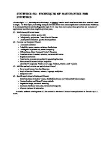
Bringing home the body of King Karl XII of Sweden. In that year, 1718, the Swedish state debt reached a high point. Painted by Gustaf Cederström (1845–1933) in 1884. Source: Nationalmuseum.

204

Historical Monetary and Financial Statistics for Sweden, Volume II

5.4.1 The period 1670–1718 The only annual figures on government debt available in printed form that we are aware of record government loans in the Riksbank, published in Sveriges Riksbank (1918). General histories of the regency period, 1660–72, refer to the period as one of peace but with weak state finances due to diminishing tax receipts. The diminishing receipts were occasioned in turn by transfers of government-owned land to the nobility before and during the regency. State finances were then improved by confiscations of the transferred land, the so-called “Reduction”, during the reign of Karl XI, 1672–97. New loans from the Riksbank began on a small scale in 1670, two years after the founding of Sveriges Riksbank, even though the Bank’s charter clearly prohibited lending to the state. Borrowing accelerated during the Scanian war (Skånska kriget, 1675–79) and debt peaked in 1685. In the next few years the loans from the Riksbank were quickly reduced by amortization. By this time, the only form of government debt seems to have been the loans from the Riksbank: “…the government’s borrowing requirements disappeared fully due to the large financial reforms of Karl XI” (Heckscher (1936), p. 372). The Great Northern War, which began in 1700 and ended with the death of Karl XII in 1718 (peace treaty in 1721), led to an accumulation of debt that cannot be followed year by year, except for the borrowing at the Riksbank (“Kronans yngre lån”). In 1719, government debt to the Riksbank made up 14 per cent of all the debt in that year, as shown in Table 5.13.

5.4.2 The period 1719–76 A National Debt Office, under the supervision of parliament, Riksens ständers kontor, was set up in 1719 to pay off the debt accumulated from 1697 to 1718 during the reign of Karl XII. Almost no new loans were taken up before 1740 and budget surpluses were used to pay off this so-called “old debt”, which was not eliminated until well into the 19th century. From 1740 the government started to raise new loans to finance the war against Russia (1741–43). The different components of the debt have been estimated separately, using available data on the debt in certain years in combination with available data on new loans and amortization. We calculate the debt recursively back in time from known amounts, using the relation: Bt–1 = Bt – Lt + AMt .

(10)

We now describe the procedures and the data we use for the old debt as well as for the new debt from 1740 onwards. The so-called “old debt” can be divided into five parts as described in Table 5.13, with the initial values in 1719. The largest part consists of: debt to the Riksbank, the insurance- and salary-notes, and the number debt. The debt to the Riksbank is known from the Bank’s annual balance sheets, given in Sveriges Riksbank (1931).

Fiscal statistics for Sweden 1670–2010

205

The other debts were left to the newly formed National Debt Office to pay off; as the Office’s main books are arranged in four-year periods, we have interpolated to estimate annual debt figures.26 Table 5.13. Composition of government debt in 1719, incurred before 1719, the “Old debt”. Swedish name Bankogälden Försäkrings- och lönesedlar

Nummergälden Kronoförpantningar

Diverse kreditorer

Explanation Loans from the Riksbank Interest bearing promissory notes paid to government employees in exchange for token money (mynttecken and myntsedlar) issued 1715–1718. Number debt. Private loans classified in 11 groups in 1719 in order of priority. Swaps of income from government properties against fixed down payment to the government for a limited period. Short-term loans from various creditors

Total 1719, dsm 6,910,796 11,049,911

24,139,180 2,301,358

2,413,481

We have calculated the initial value of debt in 1719 from known amounts in 1718. The amount of the so-called insurance notes, issued initially in 1719, was estimated; these notes were issued in exchange for token money (mynttecken and myntsedlar) to finance war from 1715 to 1718, at a devalued rate of 50 per cent. The number debt consisted of various types of loan; it included loans from churches, unpaid wages, bills etc. The name “number debt” refers to its division into 12 groups (labeled 1 to 11 and one group “without number”), which were to be paid off beginning with group 1. To this debt must be added interest arrears, which had the lowest priority. The “new debt” can be divided into five parts, as described in Table 5.14. To calculate the annual debt figures, we use information on specific new loans and the amortization of old loans given in Åmark (1961, chapter 10). Further information can be obtained by studying the debt service figures in the proposed budgets. We also make use of the inventories of total debt that were made in 1764 and 1777.27 Table 5.14. Composition of government debt incurred after 1740. Swedish name

Explanation

Bankogäld Utrikes lån Lotterilån Andra inrikes lån Lån från publika kassor

Loans from the Riksbank Foreign debt Lottery loans Other domestic debt Loans from public depositories

Start year 1743 1759 1758 1751 1731

Maximum amount, dsm (year) 49,585,997 (1772) 29,444,790 (1776) 6,650,175 (1759) 7,793,281 (1764) 4,437,240 (1764)

26 Details are given in appendix A in Fregert and Gustafsson (2005). 27 For the exact calculations and further explanations see appendix B in Fregert and Gustafsson (2005).

206

Historical Monetary and Financial Statistics for Sweden, Volume II

5.4.3 The period 1777–1857 Between 1777 and 1809, the National Debt Office presented annual debt figures, which are given in Åmark (1961). We include the debt issued by Riksgäldskontoret after 1789 in the form of short-term notes, so-called riksgäldssedlar, which became a medium of exchange. This part of the debt has the same character as the loans from the Riksbank.28 Between 1811 and 1815, foreign debt was eliminated by means of an effective default by the Swedish parliament to compensate for the losses Sweden had suffered in the Napoleonic wars (see Åmark, 1961, pp. 654–660). In addition to the debt handled by the National Debt Office, in 1808-30 the government proper had a debt to the Riksbank, which has to be added to the figures from the National Debt Office. This debt, which arose to cover expenditures for the 1808-09 war, was taken over by the National Debt Office in 1830. Only semiannual data are available for most of the period from 1815 to 1850 but this is a minor problem because there were no dramatic changes in the debt. (The only major changes were the repayment of the debt handled directly by the government proper, and for this part we have annual data from the Riksbank’s balance sheet.) To approximate the debt for the missing years we use the income-expenditure statement of the National Debt Office on new loans and amortizations.

Painting of a Russian vs. Swedish naval battle in Finnish waters. By Johan Tietrich Schoultz. Source: Wikimedia.

28 See further footnote 36 for the treatment of riksgäldssedlar.

Fiscal statistics for Sweden 1670–2010

207

5.4.4. The period 1858–2010 For this period we use the official data from the National Debt Office and add, as in the previous period, the debt of the National Board of Trade. The total debt is presented in the appendix and in Figure 5.4.29 Between 1923/24 and 1995/96 the state budget accounts were given for broken fiscal years, beginning on July 1st, so we have chosen the debt figures at mid-year (30 June) to conform with the budget data.

5.5. The consolidated central government and fiscal seigniorage For a joint analysis of fiscal and monetary policy, it is useful to look at the consolidated central government (fiscal plus monetary branch). In particular, this enables us to calculate seigniorage revenue in a manner that is consistent with the general accounting principles presented in section 2.30 The central bank budget constraint, derived from its balance sheet and income-expenditure statement, can be written as: CB * + OS = ΔB CB + ΔB *+ CBT + OU . (11) ΔHt + ΔAt + itBt–1 + it*Bt–1 t t t t t Sources

Uses

The central bank receives funds from: new high-powered money, ΔHt; new government deposits at the central bank, ΔAt; interest income on its holdings of governCB, and non-government debt, i *B * ; and other sources, OS .31 The ment debt, it Bt–1 t t –1 t central bank uses funds to: buy domestic government bonds, BtCB; buy domestic non-government and foreign bonds, Bt*; transfer funds to the fiscal branch, CBTt; and other uses, OUt.32 Consolidation is achieved by adding the one-period budget constraints of the fiscal branch (3) and of the central bank (11),33 * *– Tt + CBTt + ΔBt + ΔHt + ΔAt + it Bt–CB 1 + it Bt–1 + OSt = = Gt + It + it Bt–1 +ΔAt + ΔBtCB + ΔBt* + CBTt + OUt .

(12)

29 Separate data for the National Debt Office and the National Board of Trade are available in appendix F in Fregert and Gustafsson (2005). 30 For a related discussion see Neumann (1992, 1996). 31 Other sources of the Riksbank (OSt) is equal to: the change in capital plus other revenues (for instance capital gains) plus the increase in deposits from other than the government (or bank deposits, included in) ΔHt plus the increase in other liabilities. 32 Other uses of the Riksbank (OUt) is equal to: the increase in other assets plus the operational costs plus its profit (not transferred to the fiscal branch). 33 See Walsh (1998, pp. 132–138) for a discussion of the consolidated budget constraint and the measurement of seigniorage in a closed economy.

208

Historical Monetary and Financial Statistics for Sweden, Volume II

Equation (12) can be simplified as:34 Public . Tt + St + ΔBtPublic = Gt + It + it Bt–1

(13)

where BtPublic = Bt – BtCB is government debt held by the public and St is seigniorage: * + (OS – OU ) . St = (ΔHt – ΔBt* ) + it*Bt–1 t t

(14)

Seigniorage represents a true revenue source for the consolidated government as it can be used to finance expenditures. It consists of the flow of new high-powered money that is not used to buy domestic non-government bonds and foreign bonds, ΔHt – ΔBt* , interest on non-government bonds, it*Bt*-1, and other net inflow to the central bank, OSt – OUt.35 Rearranging (13) gives us an expression for the consolidated budget deficit: Public ) – (T + S ) = ΔB Public . DEFtC = (Gt + It + it Bt–1 t t t

(15)

where DEFtC is the deficit of the consolidated central government. We note three differences between the consolidated and the fiscal branch deficit. First, seigniorage enters as additional revenue for the consolidated central government. Second, only interest payments to the public matter for the consolidated deficit, since the interest payments from the fiscal branch to the central bank are an internal transaction that washes out as shown by (15). Third, central bank transfers do not matter, since they also represent internal transactions as shown by (15).36 Table 5.15 shows the source-use statement for the consolidated government corresponding to Table 5.4, with the budget deficit below the line and seigniorage above the line as sources.

34 We assume that all government financial assets (A t) are held at the central bank and, for simplicity, we ignore the terms “price and volume changes” and “errors and omissions”. 35 If the central bank does not buy domestic non-government bonds or foreign bonds and if the other net inflow of the central bank is zero, seigniorage is equal to ΔHt, a common empirical measure, see for example Fischer (1982). 36 The debt in riksgäldssedlar was initially considered a public debt, but the bonds soon turned into a currency. The decision in 1803 to let the Riksbank redeem 15 out of 18 million riksdaler riksgälds against 10 million riksdaler specie, confirmed the monetization of this debt. In the consolidation, we treat the riksdaler riksgälds as loans from the central bank from the beginning in 1789 and thus they never appear as public debt. Instead their increase represents seigniorage. A small error arises from the 3 million riksdaler riksgälds not redeemed by the Riksbank and which hence should be treated as public debt. Since we cannot associate the creation of these 3 million with any specific year, we have not corrected for this.

Fiscal statistics for Sweden 1670–2010

209

Table 5.15. Fiscal and monetary branch sources and uses. Sources (Inkomster) Seigniorage = net sources = St = ( Ht – Bt* ) + it*Bt-*–1+ OSt – OUt

Uses (Utgifter)

Monetary branch (central bank) Fiscal branch

Taxes and other revenues, Tt

Current expenditures, Gt Investment, It Interest on government debt, Public it Bt–1

Budget deficit, DEFtC = ΔBtPublic Total

Total

For practical reasons, we use an alternative expression of seigniorage, obtained by combining the definition of St in (14) with the central bank budget constraint in (11):37 CB St = (ΔBtCB – ΔAt ) + (CBTt – it Bt–1 ).

(16)

Seigniorage is here expressed as the sum of fiscal branch net borrowing from the central bank, ΔBtCB – ΔAt, and transfers from the central bank to the fiscal branch CB.38 net of interest payments from the fiscal branch to the central bank, CBTt – it Bt–1 Yearly data on seigniorage, interest on public debt, consolidated deficit and the public debt are presented in the appendix.

5.6. Conclusions We have presented two sets of data: fiscal branch measures and consolidated (fiscal and monetary branch) measures. Both should be useful for macroeconomic research, particularly studies that focus on the interplay between fiscal and monetary policy. Depending on the institutional set-up, studies of causation between revenues and expenditures and the sustainability of fiscal policy may use either or both measures. The most salient feature of the data is the recent rise in government debt as a fraction of GDP. It passed 60 per cent in the late 1970s, a level that had previously 37 See appendix L in Fregert and Gustafsson (2005) and Gustafsson (2005). An additional way to Public express the seigniorage is St = Gt + It + it Bt–1 – Tt – ΔBtPublic, by equation (15). However, following the discussion in the previous section, this will not be correct due to “price and volume changes” and “errors and omissions”. 38 This measure is also used by Neumann (1992), from whom we have borrowed the term fiscal seigniorage, that is, seigniorage directly used for budget purposes. This flow measure is distinct from the extra revenue the government obtains from capital gains due to unexpected inflation, which erode the real value of the debt.

210

Historical Monetary and Financial Statistics for Sweden, Volume II

been seen only in connection with the wars of Karl XII and World War II. The fast debt build-ups in 1978–82 and 1991–94 dwarf the slow increase between 1858 and 1914, when the government borrowed in international markets to build a national railway system. Remarkable are also the steady repayments of war-induced debts, inherited from despotic kings, through budget surpluses in 1719–56 and 1810–54 under new proto-democratic constitutions. The major break in the series occurs in 1821, when published closed accounts begin. Major changes in the presentation of the budget occurred in: 1912, when the budget was unified to show only flows; 1938, when the accounts were divided into a current (working) and a capital account; 1980, when the budget was unified; and 1996, when the deficit was defined as the borrowing requirement. A test of the figures’ reliability is provided in Fregert and Gustafsson (2008, section 5). We show that the figures’ reliability increases with their nearness to the present, as indicated by the decreasing difference between the change in debt and the total budget deficit.

Fiscal statistics for Sweden 1670–2010

211

Appendix Table A5.1. Expenditures, revenues, interest payments, central bank transfers, seigniorage and debt of the Swedish central government 1670–2011 in thousands of SEK. Abbreviations below. Year

Gt + It

itBt-1

Tt

CBTt

DEFt

P itBt-1

Bt

DEFtC

St

1670

3

1671

2

-1

1672

2

0

1673

3

1

1674

10

8

1675

29

18

1676

57

29

1677

100

42

1678

115

15

1679

142

28

1680

201

59

1681

215

14

1682

193

-22

1683

196

3

1684

208

12

1685

223

15

1686

238

16

1687

160

-78

1688

100

-60

1689

106

7

1690

84

-23

1691

19

-64

1692

21

2

1693

24

2

1694

26

2

1695

26

0

1696

26

0

1697

26

0

1698

26

0

1699

26

0

1700

26

0

1701

26

0

1702

69

43

1703

154

86

1704

278

124

1705

426

147

1706

441

15

1707

737

296

1708

943

206

1709

994

51

1710

995

0

1711

995

0

1712

1,000

5

1713

998

-2

1714

992

-6

1715

1,213

221

1716

1,212

-1

BtP

212

Historical Monetary and Financial Statistics for Sweden, Volume II

Table A5.1 (cont.). Expenditures, revenues, interest payments, central bank transfers, seigniorage and debt of the Swedish central government 1670–2011 in thousands of SEK. Abbreviations below. Year

Gt + It

itBt-1

Tt

CBTt

DEFt

Bt

P itBt-1

DEFtC

St

1717

1,200

-12

1718

1,152

-48

1719

7,802

1720

7,749

-53

1721

7,703

-46

1722

1,021

70

1,143

-53

7,659

BtP

6,651

-

-93

6,608 6,563 -30

6,520

1723

1,023

70

1,187

-95

7,442

-

-122

-42

6,303

1724

1,005

70

1,190

-115

7,304

-

-74

-111

6,165

1725

967

70

1,194

-156

7,256

-

30

-256

6,024

1726

914

70

1,089

-105

7,130

-

-97

-78

5,898

1727

945

70

1,338

-323

6,976

-

-163

-230

5,744

1728

1,147

70

1,413

-197

6,837

-

-101

-166

5,605

1729

1,096

70

1,428

-262

6,634

-

-162

-170

5,472

1730

916

70

1,248

-262

6,498

-

-106

-225

5,336

1731

896

66

1,209

-247

6,241

-

-114

-199

5,154

1732

823

65

1,151

-263

6,043

-

-65

-263

4,956

1733

839

66

1,184

-279

5,859

-

-45

-300

4,772

1734

847

65

1,197

-285

5,674

-

-60

-290

4,586

1735

930

66

1,283

-288

5,481

0

-104

-249

4,394

1736

950

66

1,303

-288

5,278

0

-21

-332

4,191

1737

949

65

1,305

-291

5,078

0

-82

-274

3,991

1738

855

66

1,216

-296

4,875

0

-165

-197

3,787

1739

997

66

1,238

-175

4,744

1

-237

-3

3,656

1740

945

67

1,257

-245

4,604

2

-71

-239

3,516

1741

1,689

70

1,757

2

4,504

5

-10

-53

3,416

1742

1,506

72

1,619

-41

4,368

7

-8

-98

3,280

1743

1,471

72

1,523

19

5,189

6

978

-1,024

3,153

1744

1,326

130

1,716

-260

5,114

8

-31

-351

3,072

1745

1,103

134

1,441

-204

4,934

11

-161

-166

2,979

1746

1,174

134

1,487

-180

4,796

16

-121

-176

2,892

1747

1,767

137

1,617

286

5,004

22

158

14

2,774

1748

1,471

156

1,841

-213

4,922

23

-62

-285

2,662

1749

1,298

158

1,828

-372

4,793

22

-110

-398

2,530

1750

1,698

158

2,443

-586

4,539

23

-206

-516

2,400

1751

1,800

153

1,677

276

4,823

25

3

145

2,449

1752

1,882

168

1,806

245

4,737

26

-167

269

2,336

1753

1,567

168

1,864

-129

4,714

24

-47

-226

2,242

1753

1,620

173

1,933

-141

4,691

25

-117

-172

2,161 2,105

1755

1,645

213

1,850

7

4,714

61

-154

10

1756

1,827

136

2,046

-83

4,911

58

-43

-118

2,231

1757

2,447

136

2,211

372

5,634

56

741

-449

2,131

1758

3,306

173

2,453

1,026

6,676

68

776

145

2,413

1759

2,453

193

2,306

340

7,663

65

-62

274

3,116

1760

3,239

231

2,711

759

8,303

94

179

444

3,176

1761

3,033

257

2,687

603

8,721

103

42

407

3,365

1762

2,789

273

2,499

562

10,246

112

1,297

-896

3,619

1763

4,251

300

2,576

1,975

11,169

102

-91

1,867

4,394

1764

2,700

336

2,699

336

10,523

132

-161

294

3,923

Fiscal statistics for Sweden 1670–2010

213

Table A5.1 (cont.). Expenditures, revenues, interest payments, central bank transfers, seigniorage and debt of the Swedish central government 1670–2011 in thousands of SEK. Abbreviations below. Year

Gt + It

itBt-1

Tt

CBTt

DEFt

Bt

P itBt-1

DEFtC

St

BtP

1765

2,417

337

2,367

387

10,567

139

-83

272

3,831

1766

2,171

329

3,450

-950

10,763

127

-16

-1,136

3,718

1767

2,736

331

3,329

-262

10,546

120

-120

-354

3,603

1768

1,971

335

2,601

-295

10,025

127

-599

96

3,385

1769

1,878

121

2,352

-353

9,295

121

34

-387

2,717

1770

2,171

105

2,128

148

11,552

105

108

40

4,449

1771

2,391

181

2,717

-145

11,963

181

220

-366

4,370

1772

2,712

408

3,375

-255

12,636

180

247

-730

4,372

1773

3,065

430

2,857

638

12,536

182

306

84

4,296

1774

3,090

430

3,605

-84

12,422

183

-192

-140

4,232

1775

2,533

429

3,288

-327

13,235

183

-497

-76

5,416

1776

3,115

480

3,063

532

14,503

245

-427

724

6,951

1777

2,949

557

3,173

333

14,724

335

-208

320

7,160

1778

3,197

258

5,013

-1,558

13,585

258

79

-1,637

6,021

1779

3,401

270

3,411

260

6,895

270

-7,415

7,675

6,695

1780

3,426

244

3,225

445

6,446

244

-119

563

6,446

1781

3,303

243

3,315

231

6,328

243

1

230

6,328

1782

3,321

236

3,423

135

6,559

236

-114

248

6,559

1783

3,822

242

4,518

-455

7,799

242

-215

-241

7,799

1784

3,686

305

3,876

114

7,672

305

153

-39

7,672

1785

3,913

349

3,819

442

8,094

349

-26

468

8,094

1786

3,780

356

3,554

582

8,567

356

27

555

8,567

1787

3,863

350

3,777

436

9,720

350

-80

516

9,720

1788

3,810

389

3,767

432

10,363

389

214

218

10,363

1789

17,420

235

5,231

12,424

21,351

235

5,162

7,263

16,120

1790

13,614

947

13,662

899

22,237

947

2,839

-1,940

13,792

1791

9,532

952

9,904

581

24,261

952

-24

605

16,215

1792

14,333

872

7,482

7,723

33,507

872

2,192

5,531

23,237

1793

5,587

953

5,896

644

33,934

953

1,187

-543

22,591

1794

6,337

984

5,859

1,463

36,937

984

1,333

129

24,233

1795

5,953

871

6,659

164

34,151

871

2,055

-1,891

19,511

1796

7,630

695

6,643

1,683

32,922

695

807

875

17,463

1797

5,020

795

5,513

303

32,738

795

-1,724

2,027

18,963

1798

5,739

838

6,445

132

33,976

838

1,143

-1,011

19,098

1799

6,862

988

7,060

790

38,142

988

1,085

-295

22,105

1800

7,731

950

7,496

1,185

38,901

950

2,040

-855

20,845

1801

6,721

1,035

6,988

767

40,867

1,035

-492

1,260

22,243

1802

7,096

1,083

9,844

-1,664

42,349

1,083

813

-2,477

23,406

1803

8,606

1,136

8,987

1,246

40,248

1,136

-3,053

4,192

23,041

1804

9,451

1,023

9,950

524

36,854

1,023

-2,822

3,346

21,986

1805

9,859

1,015

11,118

-243

32,723

1,015

-1,799

1,556

20,269

1806

9,454

949

10,874

-471

30,098

949

-2,414

1,942

19,922

1807

9,837

914

10,518

233

27,576

914

-1,470

1,703

19,619

1808

25,986

945

17,917

9,013

27,984

945

488

8,524

19,668

1809

21,646

963

8,954

13,655

35,135

903

6,253

7,341

18,578

1810

17,611

1,135

12,807

5,938

41,074

720

1,683

3,841

22,497

1811

13,751

1,306

14,027

1,029

42,103

785

1,771

-1,262

22,479

1812

11,347

1,381

21,546

-8,818

33,285

795

147

-9,550

13,527

214

Historical Monetary and Financial Statistics for Sweden, Volume II

Table A5.1 (cont.). Expenditures, revenues, interest payments, central bank transfers, seigniorage and debt of the Swedish central government 1670–2011 in thousands of SEK. Abbreviations below. Year

Gt + It

itBt-1

Tt

CBTt

DEFt

Bt

P itBt-1

St

DEFtC

BtP

1813

33,047

1,044

33,131

960

34,245

439

-1,795

2,150

13,576

1814

32,650

1,036

32,454

1,231

35,476

461

2,247

-1,591

12,803

1815

13,459

1,012

20,965

-6,495

28,981

449

-2,100

-4,958

8,456

1816

15,427

747

16,632

-458

28,523

211

-2,637

1,642

9,524

1817

14,553

724

16,285

-1,008

27,515

223

-857

-653

9,540

1818

15,900

702

17,638

-1,036

26,478

236

-973

-529

8,823

1819

17,029

678

17,976

-268

26,210

249

-2,866

2,168

9,856

1820

15,542

685

17,016

-789

25,421

278

-1,367

171

10,108

1821

17,403

679

16,677

1,405

24,504

295

-1,117

2,138

9,861

1822

16,355

668

16,952

72

23,867

307

-831

542

9,850

1823

15,318

657

17,034

-1,059

17,805

320

-906

-490

3,944

1824

17,178

631

17,131

678

17,109

318

268

97

3,504

1825

16,509

618

17,671

1826

18,278

605

19,530

533

-545

17,920

315

-876

29

4,559

-1,180

17,366

312

-771

-169

4,244

1827

18,880

593

18,423

502

547

16,764

310

404

361

3,883

1828

17,276

581

17,436

528

-107

15,916

307

-893

1,040

3,276

1829

12,664

328

21,076

537

-8,620

10,073

64

-7,401

-946

3,471

1830

22,163

328

20,540

481

1,469

11,811

63

-633

2,319

5,211

1831

21,853

355

21,772

75

360

13,603

91

180

-9

7,003

1832

20,991

394

21,302

121

-39

13,333

130

-860

678

6,733

1833

20,415

397

20,938

207

-334

13,043

133

51

-442

6,443

1834

20,977

399

20,765

167

444

13,183

135

623

-276

6,583

1835

20,956

432

21,572

107

-292

13,249

168

-637

188

6,781

1836

22,774

455

22,192

746

291

12,980

196

-84

862

6,644

1837

25,484

473

24,468

1,490

11,326

220

-357

1,593

5,122

1838

24,280

418

25,043

-345

10,849

170

1,278

-1,871

4,777

1839

23,740

362

24,079

24

8,830

120

-2,589

2,369

2,890

1840

23,199

316

23,463

52

8,349

79

-1,467

1,282

2,541

1841

23,514

296

24,078

1842

23,521

343

19,873

3,467

-267

10,369

64

-2,215

1,716

4,693

525

11,515

123

2,982

789

5,971

1843

22,197

355

22,778

-225

10,209

134

2,024

-2,471

4,797

1844

20,536

348

20,923

-40

8,907

132

303

-559

3,627

1845

22,679

341

23,190

-170

9,362

130

422

-803

4,214

1846

24,233

339

25,152

-579

9,823

116

-687

-115

4,807

1847

24,222

338

24,023

907

-370

11,146

97

-1,272

1,568

6,262

1848

24,604

361

20,645

4,922

-602

12,472

141

7,267

-3,166

7,720

1849

25,776

384

26,599

-439

12,158

190

-1,677

1,044

7,538

1850

25,204

355

25,579

-19

11,408

151

-758

534

6,920

1851

27,798

309

27,760

1852

28,340

304

23,870

3,150

347

13,639

125

-283

446

9,283

1,624

12,893

125

3,206

1,388

8,669

1853

26,933

298

28,193

-961

10,828

125

-317

-817

6,736

1854

31,145

323

30,279

1,189

13,929

158

-3,979

5,003

9,969

1855

33,940

324

29,560

1856

38,852

320

38,538

1857

41,675

287

36,683

1858

50,975

270

31,527

4,050

1,500

654

12,223

158

-84

4,622

8,395

634

17,206

161

4,933

-4,458

13,510

5,280

14,091

138

-183

5,314

10,527

18,219

23,645

119

3,564

16,003

20,213

1859

49,573

486

33,540

16,519

29,051

343

1,613

14,763

25,751

1860

50,322

1,607

35,776

16,153

49,788

1,470

-3,680

19,695

46,620

Fiscal statistics for Sweden 1670–2010

215

Table A5.1 (cont.). Expenditures, revenues, interest payments, central bank transfers, seigniorage and debt of the Swedish central government 1670–2011 in thousands of SEK. Abbreviations below. Year

Gt + It

itBt-1

Tt

1861

46,967

2,308

39,013

1862

48,635

2,190

39,636

CBTt

DEFt

1,000

Bt

P itBt-1

St

DEFtC

BtP

9,262

57,060

2,181

-1,099

11,234

54,024

11,189

52,410

2,061

5,254

5,805

45,596

1863

54,804

2,379

43,543

13,639

54,695

2,076

-282

13,618

48,070

1864

61,478

2,696

44,347

19,827

67,693

2,403

2,438

17,095

61,254

1865

59,571

3,524

40,659

1866

64,215

3,992

42,522

5,000

17,436

78,248

3,239

4,405

17,746

70,820

25,685

91,004

3,662

1,503

23,852

83,149

1867

47,872

4,541

38,638

3,400

10,375

99,672

4,170

2,573

10,831

91,160

1868

49,600

5,240

38,658

1,800

14,381

110,663

4,817

610

15,149

104,131

1869

49,670

5,272

39,666

1,500

13,776

114,923

4,933

1,696

13,241

107,866

1870

51,979

5,393

49,819

3,500

4,053

118,616

5,073

126

7,106

111,742

1871

52,325

5,634

58,681

1,500

-2,222

123,020

5,310

1,341

-2,387

116,123

1872

59,757

5,880

62,577

1,351

1,710

124,302

5,555

3,449

-714

117,376

1873

65,977

5,534

72,313

-

-802

121,113

5,236

-5,147

4,047

116,196

1874

90,557

5,642

81,292

-

14,907

130,697

5,401

-9,928

24,593

126,585

1875

91,567

6,030

79,689

500

17,408

140,360

5,804

5,868

11,815

137,443

1876

93,417

7,108

83,732

1,250

15,544

176,356

6,954

181

16,459

173,494

1877

92,670

8,093

82,281

1,300

17,182

182,343

7,955

8,710

9,634

175,585

1878

98,316

8,884

79,823

900

26,478

212,734

8,597

-4,010

31,100

210,008

1879

86,686

9,588

71,207

1,350

23,717

220,482

9,442

6,966

17,956

214,406

1880

78,822

9,698

81,026

1,300

6,194

230,542

9,341

1,340

5,796

222,663

1881

81,623

9,126

87,208

1,185

2,356

234,902

8,533

-2,533

5,481

227,505

1882

72,790

9,448

85,853

1,250

-4,865

229,092

9,046

-2,181

-1,836

223,243

1883

77,785

9,196

87,644

1,600

-2,263

228,013

8,922

2,993

-3,930

221,589

1884

77,240

9,449

88,666

1,300

-3,277

230,347

9,156

-4,879

2,609

225,897

1885

81,410

9,633

88,644

1,300

1,100

247,210

9,437

2,073

130

242,084

1886

88,333

10,011

84,560

1,200

12,584

245,949

9,756

406

13,122

241,244

1887

90,154

9,676

81,114

-

18,716

246,109

9,464

1,530

16,974

241,048

1888

85,050

9,761

92,861

1,250

699

265,034

9,527

-1,720

3,436

260,875

1889

86,111

10,151

98,965

-

-2,703

259,054

9,938

3,685

-6,601

254,140

1890

87,641

10,983

102,146

1,300

-4,822

259,653

10,638

1,916

-5,783

253,036

1891

98,684

9,779

98,017

1,300

9,146

265,413

9,477

-2,335

12,479

260,822

1892

97,837

9,984

95,494

1,850

10,478

274,047

9,791

2,981

9,154

268,845 274,085

1893

98,452

10,329

99,495

1,750

7,536

278,811

10,118

2,583

6,492

1894

98,401

10,544

113,316

2,801

-7,173

293,292

10,330

-3,858

-727

288,858

1895

94,923

10,456

119,121

2,480

-16,222

287,647

10,290

-84

-13,824

282,653

1896

123,946

10,269

121,780

2,340

10,095

292,878

10,079

1,687

10,558

287,907

1897

108,910

10,086

136,451

2,700

-20,155

290,750

9,913

-1,940

-15,687

285,813

1898

117,477

10,028

144,023

1,800

-18,317

286,920

9,838

3,548

-20,256

282,778

1899

132,797

10,456

153,516

2,000

-12,263

319,724

10,304

16,722

-27,137

315,676

1900

149,593

10,905

153,359

7,138

343,090

10,759

-59

7,052

340,185

1901

160,508

12,276

143,636

29,148

354,277

12,152

-5,736

34,760

352,061

1902

171,354

12,192

147,398

2,000

34,149

354,040

12,111

-9,256

45,323

351,190

1903

171,997

12,121

183,177

2,716

-1,775

352,511

12,008

-22,388

23,217

350,671

1904

190,373

12,056

185,985

3,285

13,159

391,190

11,976

3,532

12,832

389,390

1905

193,369

13,411

194,613

4,000

8,166

412,243

13,352

-1,870

13,978

410,443

1906

198,385

13,301

188,519

5,100

18,066

426,907

13,228

13,091

10,003

425,107

1907

219,597

14,693

208,755

5,350

20,186

468,102

14,622

30,570

-5,104

467,037

1908

252,441

17,133

196,096

6,400

67,077

519,071

17,099

-4,903

78,346

519,071

216

Historical Monetary and Financial Statistics for Sweden, Volume II

Table A5.1 (cont.). Expenditures, revenues, interest payments, central bank transfers, seigniorage and debt of the Swedish central government 1670–2011 in thousands of SEK. Abbreviations below. Year

Gt + It

itBt-1

Tt

CBTt

DEFt

Bt

P itBt-1

St

DEFtC

BtP

1909

257,775

18,585

206,570

8,675

61,115

554,173

18,585

-21,944

91,734

554,173

1910

250,573

19,411

236,001

8,323

25,661

543,383

19,411

15,616

18,368

543,384

1911

251,235

19,140

235,768

6,256

28,350

611,959

19,140

8,340

26,266

611,959

1912

224,878

22,511

223,265

6,399

17,725

607,964

22,511

-19,113

43,237

607,964

1913

230,019

22,697

239,891

6,311

6,514

648,287

22,697

-16,288

29,113

648,287

1914

237,197

25,438

234,934

7,058

20,643

744,455

25,438

11,046

16,655

741,200

1915

375,554

30,840

356,682

8,800

40,912

854,871

30,631

-346

49,849

848,895

1916

391,638

36,193

406,547

8,760

12,525

993,246

35,862

-21,636

42,590

992,644

1917

598,720

44,056

618,007

8,120

16,648

1,149,226

44,024

-12,018

36,754

1,141,226

1918

1,490,966

59,391

817,905

-

732,451

1,656,179

58,898

56,321

675,637

1,653,450

1919

784,003

59,480

862,038

-

-18,555

1,566,998

59,237

-93,717

74,918

1,564,086

1920

844,366

61,874

834,563

-

71,677

1,496,524

61,746

50,289

21,261

1,494,149

1921

1,014,690

64,216

759,162

-

319,744

1,510,987

64,112

-165,983

485,622

1,507,335

1922

826,130

72,231

648,592

3,500

246,270

1,551,464

71,932

-59,973

309,444

1,548,290

1923

360,679

34,288

260,515

12,000

122,452

1,566,441

34,216

221,224

-86,844

1,555,751

1923/24

658,698

81,431

647,503

16,000

76,626

1,634,038

81,195

-29,291

121,681

1,620,273

1924/25

670,994

77,286

620,650

14,000

113,630

1,734,032

76,740

9,294

117,790

1,721,061

1925/26

661,909

81,072

638,167

15,500

89,313

1,735,286

80,308

108,792

-4,742

1,722,335

1926/27

681,977

83,372

656,938

16,000

92,411

1,812,799

82,666

20,146

87,559

1,802,063

1927/28

625,009

87,068

691,131

16,200

4,746

1,825,572

86,464

-50,148

70,489

1,814,554

1928/29

680,415

86,626

718,516

13,900

34,625

1,835,170

86,217

-5,803

53,918

1,829,122

1929/30

684,193

85,997

761,466

17,000

-8,277

1,800,846

85,176

59,654

-51,752

1,778,714

1930/31

704,202

82,439

763,844

19,000

3,797

1,845,644

81,624

-53,554

75,536

1,842,625

1931/32

774,045

81,258

720,482

16,000

118,821

2,155,333

80,970

287,465

-152,932

1,936,913

1932/33

967,400

91,650

726,946

14,000

318,105

2,358,532

86,920

-13,068

340,442

2,098,455

1933/34

842,101

99,296

755,551

27,000

158,846

2,348,962

91,674

-62,563

240,788

2,197,901

1934/35

1,004,607

97,881

895,847

7,000

199,640

2,487,099

92,906

-90,354

292,020

2,358,460

1935/36

962,583

94,457

991,005

4,250

61,784

2,387,183

92,191

-90,392

154,160

2,358,683

1936/37

1,009,475

91,928

1,146,952

2,750

-48,299

2,236,798

91,437

32,529

-78,569

2,234,798

1937/38

1,213,862

88,236

1,290,893

3,900

7,305

2,430,242

87,951

-136,984

147,904

2,389,142

1938/39

1,486,834

91,144

1,440,346

1,500

136,132

2,633,617

89,782

12,802

123,468

2,481,515

1939/40

2,786,450

98,286

1,849,329

-

1,035,407

3,625,020

92,010

910,985

118,146

2,957,677

1940/41

3,737,930

145,514

2,013,633

23,000

1,846,810

5,170,035

135,093

-155,715

2,015,105

4,334,086

1941/42

3,909,613

185,176

2,248,133

19,500

1,827,155

6,926,901

173,678

288,784

1,546,373

5,860,910

1942/43

4,276,544

226,727

2,684,105

20,000

1,799,166

8,731,848

217,210

-196,892

2,006,541

7,684,797

1943/44

4,356,234

265,213

3,096,647

9,500

1,515,300

9,773,651

259,024

6,189

1,512,422

8,652,414

1944/45

4,414,425

288,303

3,244,617

6,000

1,452,111

10,952,782

283,342

-705

1,453,855

9,757,954

1945/46

3,382,532

271,791

3,521,189

7,000

126,133

11,194,922

269,513

-438,317

569,173

10,255,515

1946/47

3,545,347

310,856

3,605,836

250,367

11,419,869

303,113

1,703,516

-1,460,892

9,047,745

1947/48

4,052,614

310,447

4,437,798

-74,737

11,486,857

268,834

196,750

-313,100

8,762,807

1948/49

4,827,908

321,157

4,953,957

1949/50

4,999,799

315,265

4,829,105

195,108

11,861,090

257,740

-183,147

314,839

9,240,913

10,000

475,960

12,072,926

261,370

-56,114

488,179

9,679,609

1950/51

5,813,800

330,521

5,805,598

15,000

323,722

12,420,618

268,920

529,244

-252,122

9,379,673

1951/52

7,229,516

342,794

7,492,224

15,000

65,087

12,329,381

283,690

-988,176

1,009,159

10,152,890

1952/53

8,506,164

297,767

7,793,157

15,000

995,774

12,531,548

255,360

-63,480

1,031,848

10,801,247

1953/54

8,843,610

339,157

8,519,693

15,000

648,074

13,586,656

309,324

50,163

583,078

11,689,988

1954/55

9,341,974

350,145

8,891,828

15,000

785,291

14,524,089

335,565

581,251

204,459

12,239,826

1955/56

10,237,843

432,214

10,056,572

15,000

598,485

15,477,181

419,482

989,722

-388,969

12,181,411

Fiscal statistics for Sweden 1670–2010

217

Table A5.1 (cont.). Expenditures, revenues, interest payments, central bank transfers, seigniorage and debt of the Swedish central government 1670–2011 in thousands of SEK. Abbreviations below. Year

Gt + It

itBt-1

Tt

CBTt

DEFt

Bt

P itBt-1

St

DEFtC

BtP

1956/57

11,348,296

456,252

10,676,207

15,000

1,113,341

16,818,171

437,957

792,802

317,245

12,830,345

1957/58

12,729,269

569,424

12,004,033

15,000

1,279,660

18,361,740

500,048

93,601

1,131,683

14,193,271

1958/59

13,474,962

598,587

12,589,548

15,000

1,469,001

19,173,374

491,835

-795,652

2,172,901

15,740,625

1959/60

14,600,219

735,612

13,607,010

50,000

1,678,821

20,660,080

624,204

254,219

1,363,194

16,821,757

1960/61

15,395,763

863,561

16,590,675

50,000

-381,351

20,410,939

728,328

306,333

-772,917

16,210,494

1961/62

16,608,275

871,394

17,956,848

50,000

-527,178

19,573,850

734,519

-877,587

263,533

16,138,374

1962/63

18,774,523

768,056

19,769,053

100,000

-326,474

19,075,002

675,597

-305,134

-13,800

16,019,489

1963/64

20,221,163

792,136

20,827,171

100,000

86,128

19,270,222

745,644

282,112

-142,477

15,993,390

1964/65

23,574,560

849,038

24,156,689

100,000

166,908

19,251,809

815,307

-757,393

990,570

16,775,401

1965/66

27,484,465

885,246

27,914,920

100,000

354,791

19,622,132

859,987

1,349,956

-920,424

15,913,711

1966/67

31,153,422

918,823

30,290,702

150,000

1,631,543

21,434,913

885,071

1,263,855

483,936

16,560,099

1967/68

33,956,816

1,075,168

31,951,424

150,000

2,930,560

25,033,906

981,686

617,882

2,369,196

19,609,935

1968/69

36,186,948

1,296,803

34,636,101

200,000

2,647,650

27,000,980

1,194,798

-40,448

2,786,093

21,736,121

1969/70

41,024,809

1,679,259

38,687,114

200,000

3,816,953

30,959,881

1,594,523

1,588,777

2,343,440

24,250,367

1970/71

44,989,486

2,019,802

44,177,767

200,000

2,631,522

33,401,947

1,811,152

768,937

1,853,934

25,821,598

1971/72

52,025,330

1,944,822

50,103,063

200,000

3,667,089

37,209,105

1,693,230

1,653,506

1,961,991

27,985,794

1972/73

56,616,829

2,234,942

52,446,738

200,000

6,205,033

43,211,336

2,077,132

-2,607,492

8,854,714

36,650,913

1973/74

65,828,865

2,696,469

58,882,620

250,000

9,392,714

52,675,454

2,505,662

1,925,462

7,526,445

44,128,532

1974/75

76,981,191

3,738,664

69,672,245

350,000

10,697,610

63,680,071

3,328,611

6,414,698

4,222,860

48,668,673

1975/76

90,958,446

4,133,185

90,917,610

450,000

3,724,021

68,759,943

3,245,746

-7,801,129

11,087,712

61,215,363

1976/77

107,042,809

5,416,337

101,424,916

550,000

10,484,230

82,340,463

4,079,064

-108,530

9,805,487

73,961,639

1977/78

127,549,487

6,915,824

108,636,130

650,000

25,179,180

105,237,931

5,279,391

-1,839,491

26,032,239

97,790,186

1978/79

146,139,105

8,802,487

115,613,786

650,000

38,677,806

139,086,309

6,873,123

1,454,017

35,944,425

128,970,281

1979/80

164,067,546

14,508,895

127,842,813

750,000

49,983,629

192,088,176

11,728,720

7,682,431

40,271,022

171,852,176

1980/81

191,473,091

23,765,021

154,436,801

850,000

59,951,311

252,967,984

20,010,457

6,777,437

50,269,311

223,390,984

1981/82

207,439,903

27,724,094

165,130,779

2,000,000

68,033,218

319,686,000

22,805,432

16,360,338

48,754,218

270,861,000

1982/83

229,683,531

48,195,980

187,280,186

4,000,000

86,599,325

407,325,000

42,787,702

-21,475,277

106,666,325

378,630,000

1983/84

237,878,006

60,386,504

217,165,492

4,000,000

77,099,019

482,636,000

54,858,086

6,327,582

69,243,019

446,110,000

1984/85

253,902,037

75,234,268

255,595,866

5,000,000

68,540,438

559,459,000

68,832,350

-528,918

67,667,438

517,369,000

1985/86

256,152,965

66,508,793

269,437,949

5,661,000

47,562,810

596,015,000

58,380,362

40,778,569

4,316,810

515,375,000

1986/87

272,748,544

63,812,064

312,751,208

7,354,000

16,455,401

609,248,000

54,634,064

-11,138,000

25,769,401

537,812,000

1987/88

284,819,070

53,410,443

326,440,915

6,111,000

5,677,598

597,621,000

45,041,943

-1,080,500

4,500,598

525,115,000

1988/89

299,770,624

53,178,902

361,107,401

6,600,000

-14,757,876

589,712,000

46,474,402

9,361,500

-24,223,876

507,775,000

1989/90

341,590,624

63,696,173

395,552,551

6,000,000

3,734,246

582,456,000

57,672,173

-17,500,000

21,210,246

517,995,000

1990/91

387,474,767

61,033,277

396,486,593

7,000,000

45,021,452

626,698,000

54,285,277

-19,873,000

65,146,452

582,362,000

1991/92

432,629,822

60,042,701

390,025,287

7,700,000

94,947,236

710,982,000

50,478,701

-12,213,000

105,296,236

676,995,000

300,476,689

996,974,000

1992/93

534,779,861

73,090,178

370,443,351

7,300,000

230,126,689

960,611,000

59,780,678

-76,359,500

1993/94

487,959,873

94,736,213

367,424,870

9,500,000

205,771,216 1,178,643,000

87,174,713

126,684,500

81,025,216 1,090,260,000

1994/95

482,689,118

123,200,957

416,983,612

6,200,000

182,706,464 1,370,401,000

117,271,457

-10,511,500

193,488,464 1,292,800,000

1995/96

728,674,864

123,757,585

808,878,360

8,100,000

35,454,089 1,411,632,000

108,514,085

-25,699,500

54,010,089 1,352,587,000

1997

556,840,000

98,360,000

648,900,000

8,100,000

6,228,000 1,432,076,000

98,360,000

-1,459,000

6,228,000 1,378,988,000

1998

583,389,000

113,311,000

706,300,000

9,300,000

-9,700,000 1,448,859,000

113,311,000

-13,379,000

-9,700,000 1,416,017,000

1999

553,275,000

89,825,000

725,100,000

7,600,000

-82,000,000 1,374,180,000

89,825,000

-52,000

-82,000,000 1,345,182,000

2000

607,909,000

90,191,000

800,000,000

9,800,000

-101,900,000 1,279,205,000

90,191,000

632,000

-101,900,000 1,258,477,000 -38,747,000 1,156,827,000

2001

635,308,000

81,071,000

755,126,000 28,200,000,000

-38,747,000 1,156,827,000

81,071,000

6,126,000

2002

659,815,000

67,183,000

730,488,000 27,300,000,000

-3,500,000 1,160,329,000

67,183,000

29,504,000

-3,500,000 1,160,329,000

2003

666,268,000

42,015,000

661,731,000 7,500,000,000

46,600,000 1,228,741,000

42,015,000 7,500,000,000

46,600,000 1,228,741,000

2004

692,334,577

52,596,423

694,418,000 6,100,000,000

50,500,000 1,257,326,000

52,596,423 6,100,000,000

50,500,000 1,257,326,000

218

Historical Monetary and Financial Statistics for Sweden, Volume II

Table A5.1 (cont.). Expenditures, revenues, interest payments, central bank transfers, seigniorage and debt of the Swedish central government 1670–2011 in thousands of SEK. Abbreviations below. Year

Gt + It

itBt-1

Tt

CBTt

DEFt

Bt

P itBt-1

St

DEFtC

BtP

2005

699,210,000

32,561,000

745,825,000 6,700,000,000

-14,054,000 1,308,572,000

32,561,000 6,700,000,000

-14,054,000 1,308,572,000

2006

742,567,724

49,374,070

810,314,986 5,300,000,000

-18,373,192 1,269,957,000

49,374,070 5,300,000,000

-18,373,192 1,269,957,000

2007

713,340,198

47,166,370

863,716,282 4,400,000,000

-103,210,000 1,168,013,206

47,166,370 4,400,000,000

-103,210,000 1,168,013,206

2008

733,000,000

33,100,000

901,300,000 3,600,000,000

-135,200,000 1,119,000,000

33,100,000 3,600,000,000

-135,200,000 1,119,000,000 176,100,000 1,189,200,000

2009

854,600,000

31,100,000

709,500,000 5,900,000,000

176,100,000 1,189,200,000

31,100,000 5,900,000,000

2010

757,321,000

23,252,000

779,520,000 5,800,000,000

1,052,000 1,151,468,000

23,252,000 5,800,000,000

1,052,000 1,151,468,000

2011

770,100,000

34,500,000

872,400,000 6,200,000,000

-67,800,000 1,107,700,000

34,500,000 6,200,000,000

-67,800,000 1,107,700,000

Gt + It = government consumption and transfers, and government investment, itBt–1= interest payments on government bonds, Tt = government income, CBTt = central bank transfers to the fiscal P , = interest paybranch, DEFt, = total budget deficit of the fiscal branch, Bt = government debt, itBt–1 ments on government debt held by the public, St= seigniorage, DEFCt,= total deficit of the consolidated government, BtP= government debt held by the public.

Fiscal statistics for Sweden 1670–2010

219

Data sources Debt Åmark, K (1961), Sveriges statsfinanser 1719–1809, Norstedt & Söners förlag, Stockholm. Ekonomistyrningsverket, (1998–2012), yearly, Statsbudgetens utfall. Rikets ständers revisorer, [18--]–1866. ‘Rikets höglof. Ständers år ... församlade revisorers berättelse om granskningen af Riksgälds-kontorets tillstånd och förvaltning’, in Bihang till samtlige riksståndens protokoll (1866 i: Bihang till Riksdagens protokoll ... 1867, samling 2, afd. 1), Stockholm. Simonsson, K G, (1918), ‘Statistiska tabeller 1668–1718’, Bilaga I, in Sveriges Riksbank 1668–1924 (1918–1931), Vol. I, Norstedt and Sveriges Riksbank, Stockholm. Sveriges Riksbank (1931), ‘Statistiska tabeller 1668–1924’, in Sveriges Riksbank 1668– 1918/1924. Bankens tillkomst och verksamhet, Vol. V, Norstedt and Sveriges Riksbank, Stockholm. Riksdagens revisorer, (1868–1911), ‘Riksdagens år ... församlade revisorers berättelse om granskningen av Riksgäldskontorets tillstånd och förvaltning’, in Bihang till Riksdagens protokoll ... samling 2, Stockholm. Riksgäldskontoret, (1920–1980/81), yearly, Årsbok. Riksgäldskontoret, (1982/83–1997), yearly, Statistical Yearbook. Riksgäldskontoret, (1982/83–1997), yearly, Annual report. Revenues and expenditures Åmark, K (1961), Sveriges statsfinanser 1719–1809, Norstedt & Söners förlag, Stockholm. Ekonomistyrningsverket, (1998–2012), yearly, Statsbudgetens utfall. Rathsman, C N (1855), Underdånigt betänkande till Kongl. Maj:t angående uppgjord jemförelse emellan svenska folkets skatter samt stats- och riksgälds-verkens utgifter vid början af 1809 och 1810 års riksdag samt enehanda skatter och utgifter vid 1850 års slut: afgifvet den 4 juni 1855, Stockholm. Rikets ständers revisorer, ([18--]–1866), ‘Rikets höglof. Ständers år ... församlade revisorers berättelse om granskningen af Riksgälds-kontorets tillstånd och förvaltning’, in Bihang till samtlige riksståndens protokoll (1866 i: Bihang till Riksdagens protokoll ... 1867, samling 2, afd. 1), Stockholm. Rikets ständers revisorer, (1817–1818), Tabellbilaga Litt B och Litt C till nr 9 i Bihang till samtlige riksståndens protokoll, 2:dra samlingen, Stockholm. Riksdagens revisorer, (1868–1911), ‘Riksdagens år ... församlade revisorers berättelse om granskningen av Riksgäldskontorets tillstånd och förvaltning’, in Bihang till Riksdagens protokoll ... samling 2, Stockholm. Riksrevisionsverket, (1960/61–1979/80), yearly, Budgetredovisning för budgetåret. Riksrevisionsverket, (1980/81–1997), yearly, Statsbudgetens utfall.

220

Historical Monetary and Financial Statistics for Sweden, Volume II

Riksräkenskapsverket, (1920–1959/60), yearly, Budgetredovisning för budgetåret. Statskontoret, (1821–1854), yearly, Capital-Räkning till Riks-Hufvud-boken för år … med dertil hörande tablåer och bilagor. Statskontoret, (1854–1911), yearly, Kapital-Konto till Riks-Hufvud-Boken för år … med dertil hörande tablåer och bilagor. Statskontoret, (1912–1919), yearly, Budgetredovisning för budgetåret. Seigniorage Sveriges Riksbank (1931), ‘Statistiska tabeller 1668–1924’, in Sveriges Riksbank 1668–1918/1924. Bankens tillkomst och verksamhet, Vol. V, Norstedt and Sveriges Riksbank, Stockholm. Sveriges Riksbank, (1908–1977), yearly, Årsbok. Sveriges Riksbank, (1978–2000), yearly, Statistisk årsbok. Sveriges Riksbank, (2001–2003), yearly, Årsredovisning. Nominal GDP Edvinsson, R (2014), ‘The Gross Domestic Product of Sweden within present borders 1620–2012’, in Edvinsson, R, T Jacobson, and D Waldenström (eds.), Historical Monetary and Financial Statistics for Sweden, volume 2: House Prices, Stock Returns, National Accounts, and the Riksbank Balance Sheet, 1620–2012, Sveriges Riksbank and Ekerlids förlag, Stockholm.

Fiscal statistics for Sweden 1670–2010

221

References Åmark, K (1961), Sveriges statsfinanser 1719–1809, Norstedt & Söners förlag, Stockholm. Barro, R (1987), ‘Government spending, interest rates, prices, and budget deficits in the United Kingdom 1701–1918’, Journal of Monetary Economics, Vol. 20, pp. 221–245. Blejer, M, and A Cheasty (1991), ‘The measurement of fiscal deficits: Analytical and methodological issues,’ Journal of Economic Literature, Vol. 29, pp. 1644–1678. Dahmén, E (ed.) (1989), Upplåning och utveckling. Riksgäldskontoret 1789–1989, Allmänna förlaget, Stockholm. Edvinsson R (2010), ‘The Multiple Currencies of Sweden-Finland 1534–1803’, in Edvinsson, R, T Jacobson, and D Waldenström (eds.), Exchange Rates, Wages and Prices 1277–2008, Ekerlids förlag and Sveriges Riksbank, Stockholm. Edvinsson, R, and J Söderberg, (2010), ‘The Evolution of Consumer Prices 1290– 2008’, in Edvinsson, R, T Jacobson, and D Waldenström (eds.), Exchange Rates, Wages and Prices 1277–2008, Ekerlids förlag and Sveriges Riksbank, Stockholm. Fischer, S (1982), ‘Seigniorage and the case for a national money,’ Journal of Political Economy, Vol. 90, pp. 295–313. Fregert, K, and R Gustafsson (2005), ‘Fiscal statistics for Sweden 1719–2003. Appendices’ Working paper no 40, Department of Economics, Lund University, http://swopec.hhs.se. Fregert, K, and R Gustafsson (2008), ‘Fiscal statistics for Sweden 1719–2003’, Research in Economic History, Vol. 25, pp. 169–224. Fregert, K, and L Jonung (1996), ‘Inflation and switches between specie and paper standards in Sweden 1668–1931: A public finance interpretation’, Scottish Journal of Political Economy, Vol. 43, pp. 444–467. Heckscher, E F (1936), Sveriges ekonomiska historia från Gustav Vasa, Vol. I:2, Albert Bonniers förlag, Stockholm. Heckscher, E F (1942), De svenska penning-, vikt och måttsystemen, P.A. Norstedt och Söner, Stockholm. Jörberg, L, A History of Prices in Sweden 1732–1914, Vol. 2, GWK Gleerup, Lund. Lane, J, and S Back (1989), Den svenska statsbudgeten, SNS förlag, Stockholm. Neumann, M J (1992), ‘Seigniorage in the United States: How much does the U.S. government make from money production’, Review - Federal Reserve Bank of St. Louis Vol. 74, pp. 29–40. Neumann, M J, (1996), ‘A comparative study of seigniorage: Japan and Germany,’ Bank of Japan Monetary and Economic Studies, Vo. 14, pp. 104–142. Reinhart C M, and K S Rogoff (2009), This Time Is Different: Eight Centuries of Financial Folly, Princeton University Press, Princeton. Riksgäldskontoret (2002), ‘Statsskulden – hur och av vem ska den mätas och redovisas?’, Regeringsrapport, Dnr 2002/104. Simonsson, K G (1918), ‘Statistiska tabeller 1668–1718’, Bilaga I, in Sveriges Riks-

222

Historical Monetary and Financial Statistics for Sweden, Volume II

bank 1668–1924 (1918–1931), Vol. I, Norstedt and Sveriges Riksbank, Stockholm. Stuart, J, and M Rystedt (1905), Handbok öfver statsverkets jemte dertill hörande fonders medelsförvaltning, Stockholm. Walsh, C (1998), Monetary Theory and Policy, MIT Press, Boston.