3
Basic Valence Bond Theory
3.1 WRITING AND REPRESENTING VALENCE BOND WAVE FUNCTIONS 3.1.1
VB Wave Functions with Localized Atomic Orbitals
After looking at the VB outputs for the simple two-center/two-electron (2e/2c) bond, let us get used to the theory by applying it to these bonds to start with. A VB determinant is an antisymmetrized wave function � � that may or may not also be a proper spin eigenfunction. For example, �ab¯ � in Equation 3.1 is a determinant that describes two spin�orbitals a and b, each having one electron; the bar over the b orbital means a b spin, and the absence of a bar means an a spin: � � �ab¯ � ¼ p1ffiffiffifað1Þbð2Þ½að1Þbð2Þ� � að2Þbð1Þ½að2Þbð1Þ�g ð3:1Þ 2 The parenthetical numbers 1 and 2 are the electron indexes. By itself, this is not a proper spin-eigenfunction. However, by mixing with �determinant � �ab ¯ � there will result two spin-eigenfunctions, one having a singlet coupling and shown in Equation 3.2, the other displaying a triplet situation in Equation 3.3. In both cases, the normalization constants are omitted for the time being. � � � � ¯ � FHL ¼ �ab¯ � � �ab ð3:2Þ � � � � ¯ � CT ¼ �ab¯ � þ �ab ð3:3Þ If a and b are the respective AOs of two hydrogen atoms, FHL in Equation 3.2 is nothing else but the historical wave function used in 1927 by Heitler and London (1) to treat bonding in the H2 molecule, hence the subscript descriptor HL. This wave function displays a purely covalent bond in which the two hydrogen atoms remain neutral and exchange their spins (this singlet pairing is represented henceforth by the two dots connected by a line as 1 in Scheme 3.1). CT in Equation 3.3 represents a repulsive triplet interaction (2) between two hydrogen atoms having electrons with parallel spins. A Chemist’s Guide to Valence Bond Theory, by Sason Shaik and Philippe C. Hiberty Copyright # 2008 John Wiley & Sons, Inc.
40
WRITING AND REPRESENTING VALENCE BOND WAVE FUNCTIONS
H•—•H 1
H↑ ↑H
H– H+
H+ H–
3
4
2
41
Scheme 3.1
�The� other� VB� determinants that one can construct in this simple 2e/2c cases are �aa¯ � and �bb¯ � , corresponding to the ionic structures 3 and 4, respectively. Both ionic structures are spin-eigenfunctions and represent singlet-spin pairing. Note that the rules governing the spin multiplicities and the generation of spineigenfunctions from combinations of determinants are the same in VB and MO theories. In a simple 2e case, it is easy to distinguish triplet from singlet eigenfunctions by factorizing the spatial function from the spin function: the singlet spin eigenfunction is antisymmetric with respect to electron exchange, while the triplet is symmetric. Of course, the spatial parts behave in precisely the opposite manner, to keep the complete wave function antisymmetric. For example, the singlet spin function is a(1)b(2) � b(1)a(2), while the triplet is a(1)b(2) + b(1)a(2) in Equations 3.2 and 3.3. Note that in Equations 3.2 and 3.3, the complete wave functions are written in an isomorphic manner to the spin wave functions; the singlet HL structure has a negative sign between the determinants as in the corresponding spin function, while the triplet structure has a positive sign as in the corresponding spin function. Keeping in mind this isomorphic relation between the full wave function, in terms of Slater determinants, the corresponding spin function may come in handy for more complicated VB cases. While the H— H bond in H2 was considered as purely covalent in Heitler and London’s paper (1) (Eq. 3.2 and Structure 1), as we saw in Chapter 2, the exact description of H2 or any homopolar bond (CVB-full) involves a small contribution of the ionic structures 3 and 4, which mix by configuration interaction (CI) in the VB framework. Typically, for homopolar and weakly polar bonds, the weight of the purely covalent structure is 75%, while the ionic structures share the remaining 25%. By symmetry, the wave function maintains an average neutrality of the two bonded atoms (Eq. 3.4). �� � � �� �� � � �� ¯ � þ m �aa¯ � þ �bb¯ � l > m ð3:4aÞ CVB�full ¼ l �ab¯ � � �ab Ha � Hb � 75% ðHa ��� Hb Þ þ 25% ðHa � Hb þ þ Ha þ Hb � Þ
ð3:4bÞ
For convenience and to avoid confusion, we will symbolize a purely covalent bond between A and B centers as A� —� B, while the notation A— B will be employed for a composite bond wave function like the one displayed in Equation 3.4. In other words, A— B refers to the ‘‘real’’ bond while A� —� B designates its covalent component. 3.1.2
Valence Bond Wave Functions with Semilocalized AOs
One inconvenience of the expression of CVB-full (Eq. 3.4) is its relative complexity compared to the simple Heitler�London function (Eq. 3.2).
42
BASIC VALENCE BOND THEORY
Coulson and Fischer (2) proposed an elegant way that combines the simplicity of FHL with the ‘‘completeness’’ of CVB-full in terms of the contributing VB structures. In the Coulson�Fischer wave function, CCF, the 2e bond is described as a formally covalent singlet coupling between two orbitals wa and wb, which are optimized with freedom to delocalize over the two centers. This is exemplified below for H2 (once again dropping the normalization factors): � � � � ¯ a wb � ¯ b � � �w CCF ¼ �wa w ð3:5aÞ wa ¼ a þ eb
ð3:5bÞ
wb ¼ b þ ea
ð3:5cÞ
Here, a and b are purely localized AOs, while wa and wb are slightly delocalized or ‘‘semilocalized’’. In fact, experience shows that the Coulson�Fischer orbitals wa and wb, which result from the optimization of the coefficient e by energy minimization, are generally not very delocalized (e < 1), and as such they can be viewed as ‘‘distorted’’ orbitals that remain atomic-like in nature. However, minor as this may look, the slight delocalization renders the Coulson�Fischer wave function equivalent to the VB-full wave function (Eq. 3.4a) with the three classical structures. A straightforward expansion of the Coulson�Fischer wave function leads to the linear combination of the classical structures in Equation 3.6. � � � � � � � � ¯ �Þ þ 2eð�aa¯ � þ �bb¯ �Þ CCF ¼ ð1 þ e2 Þð�ab¯ � � �ab ð3:6Þ Thus, the Coulson�Fischer representation keeps the simplicity of the covalent picture while treating the covalent�ionic balance by embedding the effect of the ionic terms in a variational way, through the delocalization tails. The Coulson�Fischer idea was subsequently generalized to polyatomic molecules and gave rise to the GVB and SC methods, which were mentioned in Chapter 1 and will be discussed later. 3.1.3
Valence Bond Wave Functions with Fragment Orbitals
Valence bond determinants may involve fragment orbitals (FO) instead of localized or semilocalized AOs. These fragment orbitals may be delocalized, for example, some MOs of the constituent fragments of a molecule. The latter option is an economical way of representing a wave function that is a linear combination of several determinants based on AOs, much as MO determinants are linear combinations of VB determinants (see below). Suppose, for example, that one wanted to treat the recombination of the CH3� and H� radicals in a VB manner, and let (w1 � w5) be the MOs of the CH3� fragment (w5 being singly occupied), and b the AO of the incoming hydrogen. The covalent VB function that describes the active C— H bond in our study just couples the w5 and b orbitals in a singlet manner, and is expressed as in Equation 3.7: � � CðH3 C��� HÞ ¼ �w1 w1 w2 w2 w3 w3 w4 w4 w5 b¯ � � jw1 w1 w2 w2 w3 w3 w4 w4 w5 bj ð3:7Þ
WRITING AND REPRESENTING VALENCE BOND WAVE FUNCTIONS
43
in which w1 � w4 are fully delocalized over the CH3 fragment. Even the w5 orbital is not a pure AO, but may involve some tails on the hydrogens of the CH3 fragment. It is clear that this option is conceptually simpler than treating all the C— H bonds in a VB way, including those three bonds that are intact during the recombination reaction. 3.1.4
Writing Valence Bond Wave Functions Beyond the 2e/2c Case
Rules for writing VB wave functions in the polyelectronic case are just extensions of the rules for the 2e/2c case above. First, let us consider butadiene 5 in Scheme 3.2, and restrict the description to the p system. O
4
2
5
NH2
C H
3
1
6
7
Scheme 3.2
Denoting the p AOs of the C1-C4 carbons by a,b,c, and d, respectively, the fully covalent VB wave function for the p system of butadiene displays two singlet couplings: one between a and b, and one between c and d. It follows that the wave function can be expressed in the form of Equation 3.8, as a product of the bond wave functions. � � ¯ ¯ � Cð5Þ ¼ �ðab¯ � abÞðc d¯ � cdÞ ð3:8Þ Upon expansion of the product, one gets a sum of four determinants as in Equation 3.9. � � � � � � � � ¯ � � �ab ¯ cd¯ � þ �ab ¯ cd ¯ � Cð5Þ ¼ �ab¯ cd¯ � � �ab¯ cd ð3:9Þ The product of bond wave functions in Equation 3.8, involves so-called perfect pairing, whereby we take the Lewis structure of the molecule, represent each bond by a HL bond, and finally express the full wave function as a product of all these pair-bond wave functions. As a rule, such a perfectly paired polyelectronic VB wave function having n bond pairs will be described by 2n determinants, displaying all the possible 2 � 2 spin permutations between the orbitals that are singlet coupled. The above rule can readily be extended to other polyelectronic systems, like the p system of benzene (6), or to molecules bearing lone pairs as in formamide (7). In this latter case, calling n, c, and o, respectively, the p atomic orbitals of nitrogen, carbon, and oxygen, the VB wave function describing the neutral covalent structure is given by Equation 3.10: � � � � ¯ � Cp ð7Þ ¼ �nn¯ co¯ � � �nn¯ co ð3:10Þ In any one of the above cases, improvement of the wave function can be achieved by using Coulson�Fischer orbitals that take into account ionic
44
BASIC VALENCE BOND THEORY
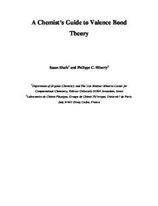
contributions to the bonds. It should be kept in mind that the number of determinants grows exponentially with the number of covalent bonds (recall, this number is 2n; n being the number of bonds). Hence, eight determinants are required to describe a Kekul´e structure of benzene, and the fully covalent and perfectly paired wave function for methane is made of 16 determinants. This underscores the incentive of using FOs rather than pure AOs, as much as possible, as has been done above (Eq. 3.7). Using FOs to construct VB wave functions is also appropriate when one wants to fully exploit the symmetry properties of the molecule. For example, we can describe all the bonds in methane by constructing group orbitals of the four hydrogens. Subsequently, we can distribute the eight bonding electrons of the molecule into these FOs as well as into the 2s and 2p AOs of carbon. Then, we can pair up the electrons using orbital symmetry-matched FOs, as shown by the lines connecting these orbital�pairs in Fig. 3.1. The corresponding wave function can be written as the following product of bond pairs: � � CðCH4 Þ ¼ �ð2s ws � ws 2sÞð2px wx � wx 2px Þð2py wy � wy 2py Þð2pz wz � wz 2pz Þ� ð3:11Þ In this representation, each bond pair is a delocalized covalent two-electron bond, written as a HL-type bond. The VB method that deals with fragment orbitals (FO�VB) is particularly useful in high symmetry cases, for example, ferrocene and other organometallic complexes. Some of its merits are further illustrated at the end of this chapter.
pz py px ϕx
ϕy
ϕz
ϕs
2s
Ψ VB (C H 4 )
FIGURE 3.1 A VB representation of methane using delocalized FOs. Each line that connects two orbitals represents a bond pair.
OVERLAPS BETWEEN DETERMINANTS
45
3.1.5 Pictorial Representation of Valence Bond Wave Functions by Bond Diagrams Since we agreed that a bond needs not necessarily involve only two AOs on two centers, we must agree on some pictorial representation of a bond. This bond diagram is in Fig. 3.2, and shows two spin-paired electrons in general orbitals w1 and w2, by a line connecting these orbitals. This bond diagram represents the wave function in Equation 3.12 Cbond ¼ jw1 w2 j � jw1 w2 j
ð3:12Þ
where the orbitals can take any shape; the wave function can involve two centers with localized AOs, or two Coulson�Fischer orbitals with delocalization tails, or FOs that span a few centers. In the case of localized orbitals, the bond-diagram represents the full-VB wave function, namely, it implicitly involves the corresponding ionic structures by shifting electrons between the pairs of coupled orbitals. ϕ2
ϕ1
FIGURE 3.2 A generic bond diagram representation of two spin-paired electrons in orbitals w1 and w2. The bond pair is indicated by a line connecting the orbitals.
3.2
OVERLAPS BETWEEN DETERMINANTS
A VB calculation is nothing else than a configuration interaction in a space of structures made of AO- or FO-based determinants. As these are in general nonorthogonal to each other, it is essential to derive some basic rules for calculating the overlaps between determinants. The fully general rules have been described in detail elsewhere (3) and will be exemplified here on commonly encountered simple cases. A more systematic presentation can be found in Appendix 3.A.1. Let us demonstrate the procedure with VB determinants of the type V and V0 in Equation 3.1, � � � � V ¼ N �a a¯ b b¯ �; V0 ¼ N 0 �c c¯ d d¯ � ð3:13Þ where N and N0 are normalization factors. Each determinant is made of a diagonal product of spin orbitals followed by a signed sum of all the permutations of this product, which are obtained by transposing the ordering
46
BASIC VALENCE BOND THEORY
of the spin�orbitals. Denoting the diagonal products of V and V0 by cd and c0 d, respectively, the expression for cd reads: ¯ ¯ cd ¼ að1Þ að2Þ bð3Þ bð4Þ;
ð1; 2; . . . are electron indexesÞ
ð3:14Þ
and an analogous expression can be written for c0 d. � � � � The overlap between the (unnormalized) determinants �a a¯ b b¯ � and �c c¯ d d¯ � is given by Equation 3.15: � ¯ �jc c¯ d dji¼ ¯ hja a¯ b bj hcd jSP ð�1Þt Pc0 d i
ð3:15Þ
where the operator P represents a restricted subset of permutations: the ones made of pairwise transpositions between spin orbitals of the same spin, and t determines the parity, odd or even, and hence the sign of a given pairwise transposition P will be negative or positive, respectively. Note that the identity permutation is included. In this example, there are four possible permutations in the product c0 d ¯ dð3Þ dð4Þ ¯ ¯ cð3Þ dð4Þ ¯ SP ð�1Þt Pðc0 d Þ ¼ cð1Þ cð2Þ � dð1Þ cð2Þ ¯ ¯ þ dð1Þ dð2Þ ¯ ¯ �cð1Þ dð2Þ dð3Þ cð4Þ cð3Þ cð4Þ
ð3:16Þ
One then integrates Equation 3.15 by � � electron � � electron, leading to Equation 3.17 for the overlap between �a a¯ b b¯ � and �c c¯ d d¯ �: � ¯ �jc c¯ d dji¼ ¯ hja a¯ b bj S2ac S2bd � Sad Sac Sbc Sbd � Sac Sad Sbd Sbc þ S2ad S2bc
ð3:17Þ
where Sac, for example, is an overlap integral between two orbitals a and c. Generalization to different types of determinants is straightforward (3). As an application, let us obtain the overlap of a VB determinant with itself, and calculate the normalization factor N of the determinant V in Equation 3.13: � ¯ �ja a¯ b bji¼ ¯ hja a¯ b bj 1 � 2S2ab þ S4ab ð3:18Þ � � ð3:19Þ V ¼ ð1 � 2S2ab þ S4ab Þ�1=2 �a a¯ b b¯ � Generally, normalization factors for determinants are larger than unity, with the exception of those VB determinants that do not have more than one spin�orbital of each spin variety, for example, as is the case of the determinants that compose the HL wave function. For these latter determinants the normalizing factor is unity, that is, N ¼ 1.
3.3 VALENCE BOND FORMALISM USING THE EXACT HAMILTONIAN Let us turn now to the calculation of energetic quantities using exact VB theory by considering the simple case of the H2 molecule. The exact electronic
VALENCE BOND FORMALISM USING THE EXACT HAMILTONIAN
47
Hamiltonian is of course the same as in MO theory, and is composed in this case of two core terms and a bielectronic repulsion: H ¼ hð1Þ þ hð2Þ þ 1=r12
ð3:20Þ
where the h operator represents the kinetic energy and the attraction between one electron and the nuclei, and r12 is the interelectronic distance. The molecular Hamiltonian is derived from the electronic one (Eq. 3.20) by adding the nuclear repulsion, here 1/R, that is, the inverse of the distance between the nuclei. 3.3.1
Purely Covalent Singlet and Triplet Repulsive States
In the VB framework, some particular notations are traditionally employed to designate the various energies and matrix elements: � ¯ �ja bji ¯ ¼ hajhjai þ hbjhjbi þ habj1=r12 jabi Q ¼ hja bjjH ð3:21Þ � ¯ �jbaji ¯ ¼ habj1=r12 jbai þ 2Sab hajhjbi K ¼ hja bjjH ð3:22Þ � ¯ �jb aji ¯ ¼ S2 hja bj ð3:23Þ ab � � Here, Q is the electronic energy of a single determinant �ab¯ � , K is the spin exchange term that will be dealt with later, and Sab is the overlap integral between the two AOs a and b. The quantity Q + 1/R has an interesting property: This quantity is quasiconstant along the interatomic distance, from infinite distance to the equilibrium bonding distance Req of H2. It corresponds to the energy of two hydrogen atoms when brought together without exchanging their spins. Such a pseudo-state (which is not a spin-eigenfunction) is called the ‘‘quasiclassical state’’ of H2 (CQC in Fig. 3.3), because all the terms of its energy have an analogue in classical (not quantum) physics. Turning now to real states, that is, spin-eigenfunctions, the total energy of the ground state of H2, in the fully covalent approximation of Heitler�London, is readily obtained: ��� � � ��� ��� � � ��� �a b¯ � � �a¯ b� �H � �a b¯ � � �a¯ b� 1 QþK 1 Eð CHL Þ ¼ ���� ¯ �� �� ¯ �������� ¯ �� �� ¯ ���� þ ¼ þ R 1 þ S2ab R ab � ab ab � ab
ð3:24Þ
Plotting the E(CHL) curve as a function of the distance now gives a qualitatively correct Morse curve behavior (Fig. 3.3), with a reasonable bonding energy, even if a deeper potential well can be obtained by allowing further mixing with the ionic terms (Cexact in Fig. 3.3). This figure shows that, in the covalent approximation, all the bonding comes from the K terms. Thus, the physical phenomenon responsible for the bond is the resonance between the two ¯ spin arrangement patterns ab¯ and ab.
48
BASIC VALENCE BOND THEORY
E
ΨT
R HH Ψ QC
Ψ HL Ψ exact
FIGURE 3.3 Energy curves for H2 as a function of internuclear distance. The curves displayed, from top to bottom, correspond to the triplet state, CT, the quasiclassical state, CQC, the HL state, CHL, and the exact full (full CI) curve, Cexact.
The term K in Equation 3.22 has been called exchange (1), but it needs not be confused with the exchange integral in MO theory. The VB term K is composed of two contributions: One is a repulsive exchange integral (which is akin to the exchange integral of MO theory). This term is positive, but necessarily small (unlike Coulomb two-electron integrals). The second is a negative term, given by the product of the overlap Sab and an integral that is called the ‘‘resonance integral’’, itself nearly proportional to Sab . Replacing CHL by CT in Equation 3.24 leads to the energy of the triplet state, Equation 3.25. ��� � � ��� ��� � � ��� �a b¯ � þ �a¯ b� �H � �a b¯ � þ �a¯ b� 1 Q�K 1 ð3:25Þ Eð CT Þ ¼ ���� ¯ �� �� ¯ �������� ¯ �� �� ¯ ���� þ ¼ þ R 1 � S2ab R ab þ ab ab þ ab Recalling that Q + 1/R is a quasiconstant from Req to infinite distance, this quantity remains nearly equal to the energy of the separated fragments and can serve, at any distance, as a reference for the bond energy, itself having a zerobonding energy. It follows from Equations 3.24 and 3.25 that, if we neglect overlap in the denominator, the triplet state (CT in Figure 3.3) is repulsive by the same quantity (�K) as the singlet is bonding (þK). Thus, at any distance >Req, the bonding energy is about one-half of the singlet�triplet energy gap. This property will be used later in applications to reactivity problems.
VALENCE BOND FORMALISM USING AN EFFECTIVE HAMILTONIAN
3.3.2
49
Configuration Interaction Involving Ionic Terms
By using the expression of the exact Hamiltonian in Equation 3.20, the selfenergy of the ionic terms and the off-diagonal Hamiltonian matrix elements are readily obtained � ¯ �ja aji¼ ¯ hja ajjH 2hajhjai þ Jaa ð3:26Þ � ¯ �ja bji¼ ¯ ð3:27Þ hja ajjH hajhjbiþSab hajhjaiþhaaj1=r12 jabi � ¯ �jb bji¼ ¯ hja ajjH 2Sab hajhjbiþhaaj1=r12 jabi ¼ K ð3:28Þ By using these matrix elements and the calculated overlaps between determinants, the accurate VB wave function of H2 (Eq. 3.4) can be variationally determined by 3 � 3 nonorthogonal CI. 3.4 VALENCE BOND FORMALISM USING AN EFFECTIVE HAMILTONIAN The use of the exact Hamiltonian for calculating matrix elements between VB determinants leads, in the general case, to complicated expressions involving numerous bielectronic integrals, owing to the 1/rij terms. Thus, for practical qualitative or semiquantitative applications, one uses an effective molecular Hamiltonian in which the nuclear repulsion and the 1/rij terms are only implicitly taken into account, in an averaged manner. Then, one defines a Hamiltonian made of a sum of independent monoelectronic Hamiltonians, much as in simple MO theory: H eff ¼ Si hðiÞ
ð3:29Þ
where the summation runs over the total number of electrons. Here, the operator h has a meaning different from Equation 3.20 since it is now an effective monoelectronic operator that incorporates part of the electron�electron and nuclei�nuclei repulsions (3). Going back to the 4e example above (Section 3.2), the determinants V and V0 are coupled by the following effective Hamiltonian matrix element: hVjH eff jV0 i ¼ hVjhð1Þ þ hð2Þ þ hð3Þ þ hð4ÞjV0 i
ð3:30Þ
It is apparent that the above matrix element is made of a sum of four terms, which are calculated independently (also consult Appendix 3.A.1). The calculation of each of these terms, for example, the first one (h(1)), is quite analogous to the calculation of the overlap in Equation 3.17, except that the first monoelectronic overlap S in each product is replaced by a monoelectronic Hamiltonian term: � �jc c¯ d dji¼ ¯ ¯ hja a¯ b bjjhð1Þ hac Sac S2bd � had Sac Sbc Sbd � hac Sad Sbd Sbc þ had Sad S2bc ð3:31aÞ hac ¼ hajhjci; and so on
ð3:31bÞ
50
BASIC VALENCE BOND THEORY
The same type of calculation is repeated for h(2), h(3), and h(4). The obtained integrals are then summed up to get the Heff matrix element of Equation 3.30.y In Equation 3.31b, the monoelectronic integral accounts for the interaction that takes place between two overlapping orbitals. A diagonal term of the type haa is interpreted as the energy of the orbital a, and will be noted ea in the following equations. By using 3.30 and 3.31, it is easy to calculate the energy of � Equations � the determinant �a a¯ b b¯ �: ¯ ¼ N 2 ð2ea þ 2eb � 2ea S2 � 2eb S2 � 4hab Sab þ 4hab S3 Þ Eðja a¯ bbjÞ ab ab ab
ð3:32Þ
where N is the normalization factor of the determinant, shown in Equation 3.19. An application of the above rules is the calculation of the energy of a spinalternant determinant like 8 in Scheme 3.3 for butadiene. Such a determinant, in which the spins are arranged so that two neighboring orbitals always display opposite spins, is referred to as a quasiclassical (QC) state and is a generalization of the QC state that we already encountered above for H2. The rigorous formulation for its energy involves some terms that arise from permutations between orbitals of the same spins, which are necessarily nonneighbors. Neglecting interactions between nonnearest neighbors, the energy of the QC state is given by the simple expression below: ¯ ¼ ea þ eb þ ec þ ed Eðja b¯ c djÞ
ð3:33Þ
8
Scheme 3.3
Generalizing: The energy of a spin-alternant determinant is always the sum of the energies of its constituting orbitals. In the QC state, the interaction between overlapping orbitals is therefore neither stabilizing nor repulsive. This is a nonbonding state, which can be used for defining a reference state, with zero energy, in the framework of VB calculations of bonding energies or repulsive interactions. Note that the rules and formulas that are expressed above in the framework of qualitative VB theory are independent of the type of orbitals y
In all rigor, the calculation of the h(1) matrix element would necessitate the permutations of the orbital products to be generated for both determinants, leading to the generation of 16 nonidentical terms. However, these terms would be redundant with those arising from the calculation of the other h(i) matrix elements, and this is why Equation 3.31 has as few terms as it does. This detail, however, does not matter as the calculation of the h(1) matrix element alone is only an intermediate step in the calculations of the whole Heff matrix element, involving all h(i) terms, in which case it is sufficient to consider the permutations in the right-hand determinant alone, as done in Equation 3.31a and in Appendix 3.A.1.
SOME SIMPLE FORMULAS FOR ELEMENTARY INTERACTIONS
51
that are used in the VB determinants: purely localized AOs, FOs, or Coulson�Fischer semilocalized orbitals. Depending on which kind of orbitals are chosen, the h and S integrals take different values, but the formulas remain the same. 3.5
SOME SIMPLE FORMULAS FOR ELEMENTARY INTERACTIONS
In qualitative VB theory, it is customary to take the average value of the orbital energies as the origin for various quantities. With this convention, and using some simple algebra (3), one can define a reduced monoelectronic Hamiltonian matrix element between two orbitals, just as done in previous chapters with offdiagonal matrix elements between VB structures (Eq. 2.6). This reduced matrix element, bab, is nothing else but the so-called and familiar ‘‘reduced resonance integral’’: bab ¼ hab � 0:5ðhaa þ hbb ÞSab
ð3:34Þ
It is important to note that these b integrals, which we use in the VB framework, are the same as those used in simple MO models, such as extended Hu¨ckel theory. Based on the new energy scale, the sum of orbital energies is set to zero, that is: Si ei ¼ 0 ð3:35Þ In addition, since the energy of the QC determinant is given by the sum of orbital energies, its energy becomes then zero: ¯ ¼0 Eðja b¯ c djÞ
3.5.1
ð3:36Þ
The Two-Electron Bond
By application of the qualitative VB theory, Equation 3.37 expresses the HL bond energy of two electrons in AOs a and b, which belong to the atomic centers A and B. The binding energy is defined relative to the quasiclassical ¯ or to the energy of the separate atoms, which is one and the same state jabj thing within the approximation scheme. In terms of bab and Sab, noted b and S for short from now on, the two-electron bonding energy is expressed as Equation 3.37: De ðA � BÞ ¼ 2bS=ð1 þ S2 Þ
ð3:37Þ
Note that if instead of using purely localized AOs for a and b, we use semilocalized Coulson�Fischer orbitals, Equation 3.37 will no more be the
52
BASIC VALENCE BOND THEORY
simple HL bond energy, but would represent the bonding energy of the real A— B bond that includes its optimized covalent and ionic components. In this case, the origin of the energy would still correspond to the QC determinant with the localized orbitals. Unless otherwise specified, in what follows we always use qualitative VB theory in this latter convention. A
B
A
9
B
A
10
B 11
Scheme 3.4
3.5.2
Repulsive Interactions in Valence Bond Theory
By using the above definitions, one gets the following expression for the repulsion energy of the triplet state (9, in Scheme 3.4): DET ðA""BÞ ¼ �2bS=ð1 � S2 Þ
ð3:38Þ
Thus, the triplet repulsion arises due to the Pauli exclusion principle and is often referred to as Pauli repulsion. For a situation where we have four electrons on the two centers (10), VB theory predicts a doubling of the Pauli repulsion, and the following expression is obtained by complete analogy to qualitative MO theory: DEðA::BÞ ¼ �4bS=ð1 � S2 Þ
ð3:39Þ
One can in fact very simply generalize the rules for Pauli repulsion. Thus, the electronic repulsion in an AO-based determinant is equal to the quantity, DErep ¼ �2nbS=ð1 � S2 Þ
ð3:40Þ
n being the number of electron pairs with identical spins. Consider, for example, VB structures with three electrons on two centers, ðA: � BÞ and (A� :B), each being described as a single AO-based determinant (see Exercise 3.3). The interaction energy that takes place between A and B in each one of these structures by itself (e.g., 11) is repulsive and following Equation 3.40 will be given by the Pauli repulsion term in Equation 3.41: DEððA: � BÞ
and
ðA� :BÞÞ ¼ �2bS=ð1 � S2 Þ
ð3:41Þ
For an interacting system that is described by a VB structure involving more than one determinant (see Exercise 3.4), Equation 3.40 can still be applied in an approximate form if squared overlaps are neglected (i.e., S2 = 0): DErep � �2nbS Equation 3.42 will be used below in Section 3.5.4.
ð3:42Þ
SOME SIMPLE FORMULAS FOR ELEMENTARY INTERACTIONS
3.5.3
53
Mixing of Degenerate Valence Bond Structures
Whenever a wave function is written as a normalized resonance hybrid between two VB structures of equivalent energies, for example, as in Equation 3.43, the energy of the hybrid is given by the normalized self-energies of the constituent resonance structures and the interaction matrix element, H12, between the structures in Equation 3.44. C ¼ N½F1 þ F2 �; 2
2
EðCÞ ¼ 2N Eind þ 2N H12 ;
N ¼ 1=½2ð1 þ S12 Þ�1=2
H12 ¼ hF1 jHjF2 i;
ð3:43Þ
Eind ¼ EðF1 Þ ¼ EðF2 Þ ð3:44Þ
where F1 and F2 are the normalized wave functions for the individual VB structures. Such mixing causes stabilization relative to the energy of each individual (Eind) VB structure, by a quantity called ‘‘resonance energy’’ (RE): RE ¼ ½H12 � Eind S12 �=ð1 þ S12 Þ;
S12 ¼ hF1 jF2 i
ð3:45Þ
The resonance energy is nothing else but the difference between the energy of the resonance hybrid and that of a reference state. This definition is general, and the reference state is taken as any one of the two individual VB structures if they are degenerate, and as the lowest of the two if they have different energies. Equation 3.45 expresses the RE for the case where the two limiting structures F1 and F2 have equal or nearly equal energies, which is the most favorable situation for maximum stabilization. However, if the energies E1 and E2 are significantly different, then according to the usual rules of perturbation theory, the stabilization will still be finite, albeit smaller than in the degenerate case (see, e.g., the VB interaction diagram in Fig. 2.1). A typical situation, where the VB wave function is written as a resonance hybrid, is odd-electron bonding (1e or 3e bonds). For example, a 1e bond A� B is a situation where only one electron is shared by two centers A and B (Eq. 3.46), while three electrons are distributed over the two centers in a 3e bond A;B (Eq. 3.47): A� B ¼ Aþ� B $ A�þ B; �
�
A;B ¼ A :B $ A: B
CðA� BÞ ¼ Nðj � � � aj þ j � � � bjÞ ¯ þ j � � � abbjÞ ¯ CðA;BÞ ¼ N 0 ðj � � � aabj
ð3:46Þ ð3:47Þ
Simple algebra (see Exercise 3.3) shows that in both cases, the overlap between the two interacting VB structures is equal to S (the hajbi orbital overlap)z and that resonance energy follows Equation 3.48: RE ¼ b=ð1 þ SÞ ¼ De ðAþ� B $ A�þ BÞ
ð3:48Þ
z Writing F1 and F2 so that their positive combination is the resonance-stabilized one. For the 3e case, this implies that the two determinants are written in such a way that they exhibit maximum orbital and spin correspondence, as in Equation 3.47. See also, Appendix 3.4.2.
54
BASIC VALENCE BOND THEORY
Equation 3.48 also gives the bonding energy of a 1e bond. Combining Equations. 3.41 and 3.48, we get the bonding energy of the 3e bond, Equation 3.49: De ðA� :B $ A: � BÞ ¼ �2bS=ð1 � S2 Þ þ b=ð1 þ SÞ ¼ bð1 � 3SÞ=ð1 � S2 Þ ð3:49Þ These equations for odd-electron bonding energies are good for cases where the forms are degenerate or nearly so. In cases where the two structures are not identical in energy, one should use the perturbation theoretic expression (3). For more complex situations, general guidelines for derivation of matrix elements between polyelectronic determinants are given in Appendices 3.A.1 and 3.A.2. Alternatively, one could follow the protocol given in the original literature (3,4). 3.5.4
Nonbonding Interactions in Valence Bond Theory
Some situations are encountered where one orbital bears an unpaired electron in the vicinity of a bond, like 12 in Scheme 3.5. A
B•—•C
A•—•B
12
C•—•D 13
Scheme 3.5
Since the A� B� —� C structure displays a singlet coupling between orbitals b and c, Equation 3.50 gives its wave function: ¯ � jabcjÞ ¯ A� B��� C¼ Nðjabcj
ð3:50Þ
in which it is apparent that the first determinant involves a triplet repulsion (between the electrons in a and b) while the second one is a spin-alternant determinant. The energy of this state, relative to a situation where A and BC are separated, can be estimated by means of Equation 3.42, leading to Equation 3.51: EðA� B��� CÞ � ½EðA� Þ þ EðB��� CÞ� � �bS
ð3:51Þ
which means that bringing an unpaired electron in the vicinity of a covalent bond results in one-half of the full triplet repulsion (for the calculation of the exact nonbonding interaction energy between A� and B� —� C, see Exercise 3.4). This property will be used below when we discuss VB correlation diagrams for radical reactions. The repulsion is the same if we bring two covalent bonds, A� —� B and C� —� D, close to each other, as in 13: EðA��� B . . . C��� DÞ � ½EðA��� BÞ þ EðC��� DÞ� � �bS
ð3:52Þ
SOME SIMPLE FORMULAS FOR ELEMENTARY INTERACTIONS
55
Equation 3.52 can be used to calculate the total p energy of one canonical structure of a polyene, for example, 14 of butadiene (Scheme 3.6).
14
Scheme 3.6
Since there are two covalent bonds (each accounting for 2bS) and one nonbonded repulsive interaction (�bS) in this VB structure, its energy simply expresses a balance between the two corresponding energy quantities, namely: Eð14Þ � 4bS � bS ¼ 3bS
ð3:53Þ
As an application, let us compare the energies of two isomers of hexatrienes. The linear s-trans conformation can be described as a resonance between the canonical structure 15 and ‘‘long-bond’’ structures 16–18 (Scheme 3.7), where one short bond is replaced by a long one. On the other hand, the branched isomer is made of only structures 19–21, since it lacks an analogous structure to 18. It is apparent that the canonical structures 15 and 19 have the same energies (three bonds, two nonbonded repulsions in both cases), and that structures 16–18, 20, and 21 are also degenerate (two bonds, three nonbonded repulsions). Furthermore, if one omits structure 18, the matrix elements between the remaining long-bond structures and the canonical ones are all the same (see Appendix 3.A.2). Thus, elimination of structure 18 will make the two isomers isoenergetic. If, however, we take structure 18 into account, it will mix and increase, however slightly, the RE of the linear polyene that becomes thermodynamically more stable than the branched one. This subtle prediction, which is in agreement with experiment, can also be demonstrated in the framework of the Heisenberg Hamiltonian (see later).
•
• 16
15
•
•
18
17
•
•
• •
19
20
Scheme 3.7
•
•
21
56
BASIC VALENCE BOND THEORY
3.6 STRUCTURAL COEFFICIENTS AND WEIGHTS OF VALENCE BOND WAVE FUNCTIONS Once a wave function C is available and is written as a linear combination of VB structures FK, as in Equation 3.54, the major VB structures can be distinguished from the minor ones by consideration of the magnitudes of their respective coefficients. X C¼ CK FK ð3:54Þ K
More generally, one has to consider the ‘‘weights’’ of VB structures, which are quantitatively related to physical properties like electron densities, net charges, and so on. According to the popular Chirgwin�Coulson formula (5), the weight of a given structure, FK, is defined as the square of the coefficient plus one-half of the overlap population terms with all the other structures: X CK CL hFK jFL i ð3:55Þ WK ¼ L
This formula is the VB analogue of the Mulliken population in MO-based calculations. The VB weights sum to unity if the wave function C, in Equation 3.54, is normalized. However, Equation 3.55 can be used even if the FK VB structures are not normalized, or even if FK represents an AO-based determinant rather than a VB structure. In such a case, it is useful to note that with the definition of the weights as in the Chirgwin�Coulson formula, the weight of a VB structure is equal to the sum of the weights of its constituting VB determinants. Other definitions have also been proposed, such as the Lo¨wdin weights (6), Equation 3.56, and the inverse weights (7), Equation 3.57. WKLowdin ¼
X
1=2
1=2
I;J
WKINV ¼ NCK2 =ðS�1 ÞKK ;
ð3:56Þ
SKI CI SKJ CJ N ¼ 1=
X
CK2 =ðS�1 ÞKK
ð3:57Þ
K
where N is a normalization factor. All these definitions generally yield results that are consistent with one another, as can be seen in some outputs displayed in Chapter 2.
3.7 BRIDGES BETWEEN MOLECULAR ORBITAL AND VALENCE BOND THEORIES After reviewing basic elements of VB theory, we would like to create bridges between the popular and widely used MO theory and the less familiar VB
BRIDGES BETWEEN MOLECULAR ORBITAL
57
theory. The goal here is not to demonstrate that one theory is ‘‘better’’ than the other, but actually to show that by borrowing insights from MO theory, VB theory itself becomes easier to handle, more predictive and more widely applicable to chemical problems. 3.7.1 Comparison of Qualitative Valence Bond and Molecular Orbital Theories Some (not all) of the elementary interaction energies that are discussed above have also qualitative MO expressions, which in some cases match the VB expressions. In qualitative MO theory, the interaction between two overlapping AOs leads to a pair of bonding and antibonding MOs, the former being stabilized by a quantity b/(1 + S) and the latter destabilized by �b/(1 � S) relative to the nonbonding level. The stabilization� destabilization of the interacting system relative to the separate fragments are then calculated by summing up the occupancy-weighted energies of the MOs. A comparison of the qualitative VB and MO approaches is given in Table 3.1, where the energetics of the elementary interactions are expressed with both methods. It is apparent that both qualitative theories give identical expressions for the odd-electron bonds, the 4e repulsion, and the triplet repulsion. This is not surprising if one notes that the MO and VB wave functions for these four types of interaction are identical (see Exercise 3.5 and Section 3.7.3 about the relationship between MO and VB wave functions). On the other hand, the expressions for the MO and VB 2e bonding energies are different; the difference is related to the fact that MO and VB wave functions are themselves different in this case (see next Section 3.7.2). There follows a rule that may be useful if one is more familiar with MO theory than with VB. Whenever the VB and MO wave functions of an electronic state are equivalent, the VB energy can be estimated using qualitative MO theory.
TABLE 3.1 Elementary Interaction Energies in the Qualitative MO and VB Models Type of Interaction 1-electron 2-electron 3-electron 4-electron triplet repulsion 3-electron repulsion
Stabilization or Destabilization (MO Model)
Stabilization or Destabilization (VB Model)
b/(1 + S) 2b/(1 + S) b (1 � 3S)/(1 � S2) �4bS/(1 � S2) �2bS/(1 � S2)
b/(1 + S) 2bS/(1 + S2) b(1 � 3S)/(1 � S2) �4bS/(1 � S2) �2bS/(1 � S2) �2bS/(1 � S2)
58
BASIC VALENCE BOND THEORY
3.7.2 The Relationship between Molecular Orbital and Valence Bond Wave Functions What is the difference between the MO and VB descriptions of an electronic system, at the simplest level of both theories? As we will see, in the cases of 1e, 3e, and 4e interactions between two centers, there is no difference between the two theories, except for the representations that look different. On the other hand, the two theories differ in their description of the 2e bond. Once again let us take the example of H2, with its two AOs a and b, and examine the VB description first, dropping normalization factors for simplicity. As has been said already, at the equilibrium distance the bonding is not 100% covalent, and it requires some ionic component to be described accurately. On the other hand, at long distances the HL wave function is the correct state, as the ionic components necessarily drop to zero and each hydrogen atom carries one electron away through homolytic bond breaking. The HL wave function dissociates correctly, but is quantitatively inaccurate at bonding distances. Therefore, the way to improve the HL description is straightforward: by simply mixing FHL with the ionic determinants and optimizing the coefficients variationally, by CI. One then gets the wave function CVB-full, in Equation 3.4, which contains a major covalent component and a minor ionic one. Now let us turn to the MO description. Bringing together two hydrogen atoms leads to the formation of two MOs, s and s� , respectively bonding and antibonding (Eq. 3.58, dropping normalization constants). s ¼ a þ b;
s� ¼ a � b
ð3:58Þ
At the simple MO level, the ground state of H2 is described by CMO, in which the bonding s MO is doubly occupied. Expansion (see Chapter 4 for a general method in the polyelectronic case) of this MO determinant into its AO determinant constituents leads to Equation 3.59 (again dropping normalization constants): � � �� � � �� �� � � �� ¯ � ¼ �a b¯ � � �a¯ b � þ �a a¯ � þ �b b¯ � CMO ¼ �s s ð3:59Þ From Eq. 3.59, it is apparent that the first one-half of the expansion is nothing else but the Heitler�London function FHL (Eq. 3.2), while the remaining part is ionic. It follows that the MO description of the homonuclear 2e bond will always be half-covalent and half-ionic, irrespective of the bonding distance. Qualitatively, it is already clear that in the MO wave function, the ionic weight is excessive at bonding distances, and becomes absurd at long distances, where the weight of the ionic structures should drop to zero to accord with the homolytic cleavage. The simple MO description does not dissociate correctly. This is the reason why it is inappropriate for the description of stretched bonds, as, for example, those found in transition states. The remedy for this poor
BRIDGES BETWEEN MOLECULAR ORBITAL
59
description is CI, specifically the mixing of the ground configuration, s2, with the diexcited one, s� 2. The reason why this mixing re-sizes the covalent vs. ionic weights is the following: If one expands the diexcited configuration, CD, into its VB constituents, one finds the same covalent and ionic components as in Equation 3.59, but coupled with a negative sign as in Equation 3.60: �� � � �� �� � � �� ð3:60Þ CD ¼ js� s� j ¼ � �a b¯ � � �a¯ b� þ �a a¯ � þ �b b¯ � It follows that mixing the two configurations CMO and CD with different coefficients, as in Equation 3.61, will lead to a wave function CMO�CI in which the covalent and ionic components ¯ � c2 js� s� j CMO�CI ¼ c1 js sj
c1 ; c2 > 0
ð3:61Þ
have unequal weights, as shown by an expansion of CMO�CI into AO determinants in Equation 3.62: �� � � �� �� � � �� ð3:62aÞ CMO�CI ¼ ðc1 þ c2 Þ �a b¯ � � �a¯ b� þ ðc1 � c2 Þ �a a¯ � þ �b b¯ � c1 þ c2 ¼ l;
c1 � c2 ¼ m
ð3:62bÞ
Since c1 and c2 are variationally optimized, expansion of CMO�CI should lead to exactly the same VB function as CVB-full in Equation 3.4, leading to the equalities expressed in Equation 3.62 and to the equivalence of CMO�CI and CVB-full (see Exercise 3.1) The equivalence also includes the Coulson�Fischer wave function CCF (Eq. 3.5) which, as we have seen, is equivalent to the VBfull description (see Exercise 3.2). CMO 6¼ CVB ;
CMO�CI :CVB�full :CCF
ð3:63Þ
To summarize, the simple MO level describes the bond as being too ionic, while the simple VB level (Heitler�London) defines it as being purely covalent. Both theories converge to the right description when CI is introduced. The accurate description of 2e bonding is half-way in between the simple MO and simple HLVB levels; elaborated MO and VB levels become equivalent and converge to the right description, in which the bond is mostly covalent, but has a substantial contribution from ionic structures. This equivalence clearly projects that the MO�VB rivalry, discussed in Chapter 1, is unfortunate and senseless. Both VB and MO theories are not so diametrically different that they exclude each other, but rather two representations of reality, which are mathematically equivalent. The best approach is to use these two representations jointly and benefit from their complementary insight. In fact, from the above discussion of how to write a VB wave function, it is apparent that there is a spectrum of orbital representations that stretches between the fully local VB representations through semilocalized CF orbitals, to the use of delocalized fragment orbitals VB (FO�VB), and all
60
BASIC VALENCE BOND THEORY
the way to the fully delocalized MO representation (in the MO�CI language). Based on the problem at hand, the choice representation from this spectrum of possibilities should be the one that gives the clearest and most portable insight into the problem. Up to this point, we restricted ourselves to the simple case of determinants involving no more than two orbitals. However, the MO�VB correspondence is general, and in fact, any MO or MO�CI wave function can be exactly transformed into a VB wave function, provided it is a spin-eigenfunction (i.e., not a spin-unrestricted wave function). While this is a trivial matter for small determinants, larger ones require a bit of algebra and a systematic method is discussed in Chapter 4 for the interested or advanced reader.
3.7.3 Localized Bond Orbitals: A Pictorial Bridge between Molecular Orbital and Valence Bond Wave Functions The standard MO wave function involves canonical MOs (CMOs), which are permitted to delocalize over the entire molecule. However, it is well known (8,9) that an MO wave function based on CMOs can be transformed to another MO wave function that is based on localized MOs (LMOs), known also as localized bond orbitals (LBOs) (10). This transformation is called unitary transformation, and as such, it changes the representation of the orbitals without affecting the total energy or the total MO wave function. This equivalence is expressed in Equation 3.64: � � � � � � � � cmo lbo lbo . . . w . . . ¼ . . . w . . . w . . . ð3:64Þ �. . . wcmo � � � i j i j corresponds to a CMO while wlbo is an LBO. where wcmo i i A unitary transformation involves simple subtractions and additions of orbitals within the complete set of the occupied CMOs. To illustrate such a transformation, we choose a simple molecule, BeH2, for which the procedure may be done in a pictorial manner without resort to equations. Figure 3.4 shows the valence occupied CMOs of BeH2, the lowest of the two is made from the bonding combination of the 2s AO of Be and the positive combination of the 1s AOs of the two hydrogen atoms, while the higher one is the bonding orbital between the 2pz(Be) orbital and the negative combination of the 1s(H) AOs. We can now make two linear combinations of these orbitals, one negative and one positive, as in Equation 3.65, dropping normalization constants: sR ¼ wcmo þ wcmo 1 2 ;
sL ¼ wcmo � wcmo 1 2
ð3:65Þ
These linear combinations, shown on the right-hand side of Figure 3.4, are seen to generate two LBOs made from sp hybrids on the Be and the 1s AOs of the hydrogens. One of these LBOs, sR, is a two-center bonding orbital localized on the right-hand side of the molecule, while the other, sL, is equivalent to the
BRIDGES BETWEEN MOLECULAR ORBITAL
61
former, but localized on the left-hand side. Of course, since the coefficients of the hydrogens in wcmo and wcmo are not exactly equal in absolute value, the 1 2 localization is not perfect, and each LBO contains a small component out of the bonding region, called ‘‘delocalization tail’’, which is, however, very small. The wave function based on these localized orbitals possesses two doubly occupied LBOs and is completely equivalent to the starting wave function based on CMOs, as expressed in Equation 3.66: � � cmo cmo cmo � ¼ js s s s j CðBeH2 Þ ¼ �wcmo ð3:66Þ R R L L 1 w1 w2 w2 This LBO-based wave function is not a VB wave function. Nevertheless, it represents a Lewis structure, and hence also a pictorial analogue of a perfectpairing VB wave function. The difference between the LBO and VB wave functions is that the latter involves electron correlation while the former does not. As such, in a perfectly paired VB wave function, based on CF orbitals, each localized Be— H bond would involve an optimized covalent�ionic combination as we demonstrated above for H2 and generalized for other 2e bonds. In contrast, the LBOs in Equation 3.65 possess some constrained combination of these components, with exaggeration of the bond ionicity. Of course, the LBO wave function in Equation 3.65 can be upgraded to a proper VB wave function quite easily, by first localizing the vacant orbitals of BeH2, in much the same way as we just did for the occupied ones, and as illustrated in the upper right-hand side of Figure 3.4. By using these vacant
z
ϕ2∗cmo
σR*
σL*
σR
σL
ϕ1∗cmo
ϕ2cmo ϕ1cmo H Be H
FIGURE 3.4 Transformation of the valence orbitals of BeH2, from canonical MOs (left-hand side) to localized bond orbitals (right-hand side). This transformation leaves the polyelectronic Hartree�Fock function unchanged.
62
BASIC VALENCE BOND THEORY
s� -LBOs, we can improve the LBO wave function in Equation 3.66 by CI, in the same manner as discussed above for H2. Now the resulting wave function will be equivalent to a VB wave function involving two localized bond pairs with CF orbitals, and would correspond to a perfect pairing GVB wave function for the molecule. Thus, the LBO wave function can be considered qualitatively as a crude VB wave function, just one step before the improvement of the covalent�ionic components of each bond. As such, we will occasionally be using LBO-based wave function in our various applications of VB theory to chemical reactivity and as an entry to bonding in organometallic complexes. Some relevant exercises are given in the end of the chapter. For molecules involving many bonds, the localizing unitary transformations are more complicated than in the BeH2 case, and are usually done by means of a computer program. This program is available in all current ab initio codes. As there are an infinite number of unitary transformations of orbitals that leave the Slater determinant unchanged, the localizing transformations are determined so as to best satisfy some specific criteria, for example, by requiring that the total spread of the localized orbitals be minimal, as in the Foster�Boys method (9). On the other hand, it is impossible to find a set of well-localized orbitals for molecules whose electronic system is intrinsically delocalized, like benzene or, to a much lesser extent, butadiene (see Exercise 3.8). As an example of using the LMO and VB�FO concepts to gain insight into bonding in a complex molecule, we selected the organometallic compound, Fe(CO)4[h2 — C2H4] in which we intend to consider the bonding between iron and ethylene, and the stereochemistry of the molecule. Of course, the use of qualitative MO theory for this molecule would have been sufficiently simple and successful. The intention here is to illustrate that VB theory can become widely applicable by importing key insights from MO theory. Elian and Hoffman (11) showed that one can start from an octahedral complex, M(CO)6, and convert the CMOs of the complex to M-CO LBOs, which are localized along the axes of the octahedron. Subsequently, by successively removing CO ligands, they show that each ligand removal leaves behind a hybrid orbital localized on the metal and pointing along the axis of the missing site of the octahedron. The two hybrids are part of the d-block orbitals, which now has three low lying orbitals from the t2g set in the octahedron, and two hybrid orbitals that replace the eg set of the octahedron. Subsequently, this has formed the basis for the now well known ‘‘isolobal analogy’’ between organometallic and organic fragments (12). Following the Hoffmann�Elian strategy, the Fe(CO)4 fragment has two hybrids (h1 and h2) pointing toward the missing axes of the octahedron, as shown in Fig. 3.5a. Since Fe in oxidation state zero has eight valence electrons, the d-block orbitals will have a filled ‘‘t2g’’ set, and singly occupied hybrids (h1 and h2) pointing toward the missing sites of the octahedron. Now we can bring ethylene and try to bind it with Fe(CO)4. One way to do that is to use the two
BRIDGES BETWEEN MOLECULAR ORBITAL
63
localized hybrids on Fe(CO)4, to uncouple the electrons of the p-bond in ethylene, and form two new bonds using covalent and ionic structures, as we did in the chapter. Since we are interested in building bridges to MO theory, we are going to use FOs, and exploit their symmetry in order to generate the VB wave function. This is done in Fig. 3.5b, where the ‘‘t2g’’ set is omitted for clarity; first we form two linear combinations from the two localized hybrids (exactly the opposite procedure of the localization in the preceding exercises), one symmetric and one antisymmetric with respect to the plane of symmetry that includes the (CO)— Fe— (CO) axis. As amply discussed (11,12), the antisymmetric combination is dominated by the 3d orbital of iron, while the symmetric combination has a large component of 4s and 4p, Therefore, the latter orbital is higher in energy than the former. Each of these new orbitals has a single electron, capable of making two bonds with the p-electrons on ethylene. As shown in the scheme, a perfect pairing bond diagram between the two fragments requires uncoupling of the p-electrons of ethylene. Thus, in order to form the maximum number of bonds, the ethylene molecule must be promoted to a triplet pp� state, so that the electrons in the symmetry-matched orbitals can form bond pairs between the two fragments. The resulting bonding scheme describes a metallacyclopropane�iron tetracarbonyl complex. It is further seen that in order to maintain two bond pairs, the ethylene must occupy the equatorial plane of the molecule. Rotation of the ethene to the axial plane will break one bond pair (the one between p� and h1 �h2) and will encounter a significant rotational barrier (the experimental value (13) is 18�25 kcal/mol). Instant recognition of stereochemistry is one of the advantages of using FO�VB representation over AO�VB. Later we will see other advantages of the FO�VB representation. As discussed above, the bond diagram represents the HL-type coupling between the FOs, as well as the ionic structures that can be generated from them. This is done by simply shifting electrons between the orbitals that form the bond pair in the fundamental perfect-pairing diagram (see Fig. 3.5b). Some of the so generated structures are shown in Fig. 3.5c. One can see two ionic structures (Fion) that are generated by transferring one electron either from the ethylene to the Fe(CO)4 fragment or vice versa. The third structure in Fig. 3.5c is generated from the fundamental one by transferring two electrons, but this generates a no-bond wave function (Fnb), which by itself is nonbonded. The wave function of the complex will be a linear combination of the four structures in Figs. 3.5b and c. In a series of olefins, we may expect to see a spectrum of cases. For example, in a series of olefins where the singlet-to-triplet pp� excitation is gradually lowered we may see an increasing metallacyclic character up to complexes, where the C— C distance is that of a single bond. With olefins that are good electron donors, we may see a wave function dominated by a mixture of Fion(1) and Fnb, while for powerful electron acceptors, we may expect a wave function dominated by Fion(2) and Fnb.
64 (a)
(b) CO
OC OC
h2
FO-VB Diagram π* (A)
h1,2 h1+h2 (S)
Fe CO
"t2g"
h1-h2 (A)
π (S)
h1 CO OC OC
(c)
H Fe
C
H CO
π* (A) h1+h2 (S)
π* (A) h1+h2 (S) h1-h2 (A)
h1-h2 (A) π (S) ΦIon(1)
H
H
π* (A) h1+h2 (S)
h1-h2 (A)
C
π (S)
π (S) ΦIon(2)
Φnb
FIGURE 3.5 The FO�VB representation of the bonding between Fe(CO)4 and ethylene: (a) The localized hybrids of Fe(CO)4, (b) the FO�VB bond diagram that describes perfect pairing between two fragments, (c) different VB�FO contributions to the bonding due to charge transfer between the two fragments.
APPENDIX
APPENDIX
65
3.1
3.A.1.1. NORMALIZATION CONSTANTS, ENERGIES, OVERLAPS, 3.A.1 AND MATRIX ELEMENTS OF VALENCE BOND WAVE FUNCTIONS This appendix describes a scheme for enumerating VB terms in a didactic manner (3,4). The Hamiltonian that is used for calculating energies and matrix elements is the effective polyelectronic Hamiltonian H, which is expressed as a sum of monoelectronic Hamiltonians h(i), one per electron: H ¼ hð1Þ þ hð2Þ þ hð3Þ þ hð4Þ þ � � �
ð3:A:1Þ
This scheme involves no approximations and can be used to obtain all the contributing terms, if one so wishes. Let us exemplify the procedure with the following VB function, which involves a unique determinant, preceded by a normalization constant N. � � ¯ b¯ � V ¼ N �a ab ð3:A:2Þ The corresponding diagonal spin�orbital product is, ¯ ¯ cd ¼ að1Það2Þbð3Þ bð4Þ;
ð1; 2; � � � are electron indexesÞ
ð3:A:3Þ
To begin with, there are a total of 24 permutations on this diagonal element. These can be minimized by eliminating all the permutations that transpose spin�orbitals of a different spin variety (a and b), because these permutations have zero contributions to all the title quantities. We can therefore group the spin�orbitals of the determinant into two subsets and define elementary permutations that act exclusively within the subsets. From there, we can build up more complex permutations, until all the contributing permutations are included. The elementary permutations are the identity that leaves unchanged the cd of any determinant, and the permutations that cause a single pairwise transposition in the order of the spin�orbitals. The sign of the elementary permutations is given by (�1)t, where t is the number of pairwise transpositions. For the diagonal element in Equation 3.A.3 the elementary permutations are, ð�1Þt Pelem ¼ P0 ; �Pab ; �P a¯ b¯ ;
ðP0 ¼ identityÞ
ð3:A:4Þ
where the subscript of the permutation defines its applied transposition. Successive applications of the elementary permutations are used to construct more complex permutations. In this manner, we generate composite permutations that perform two, three, or more, pairwise transpositions within each spin�orbital subset, or composite permutations which perform the transpositions simultaneously on the two spin�orbital subsets. For our example, the
66
BASIC VALENCE BOND THEORY
only composite permutation is, ð�1Þt Pcomp ¼ ð�Pab Þ; ð�Pa¯b¯Þ ¼ Pab Pa¯b¯
ð3:A:5Þ
The total number of permutations that are selected by this process are then, ð�1Þt Pi ¼ P0 ; �Pab ; �Pa¯b¯; Pab Pa¯b¯
ð3:A:6Þ
Thus we have minimized the number of permutations in our example from 24 to 4. For a 6 � 6 determinant, this selection process leaves 36 of the 720 possible permutations. 3.A.1.2. 3.A.1.1
Energy and Self-Overlap of an Atomic Orbital-Based Determinants
Having the permutations, we now set a table including them (Table 3.A.1). The first column of the table lists all the permutations with their signs. The title line in the second column of the table is the diagonal spin�orbital product of Equation 3.A.3, and lined below it are all the permuted products that result after the permutations that are indicated in the first column, in each line. In the third column we list the contributions of each permutation to the energy of the determinant. Table 3.A.1 (�1)tPi (1) (2) (3) (4)
P0 �Pab �Pa¯b¯ Pab Pa¯b¯
a a¯ b a a¯ b �b a¯ a �a b¯ b b b¯ a
b¯ b¯ b¯ a¯ a¯
Energy Terms 2ea þ 2eb �ea S2ab � eb S2ab � 2hab Sab �ea S2ab � eb S2ab � 2hab Sab þ4hab S3ab
The third column of the table includes energy terms, which correspond to the following integral, hcd jhð1Þ þ hð2Þ þ hð3Þ þ hð4Þjð�1Þt Pi cd i
ð3:A:7Þ
Accordingly, the total energy contribution, in each of the table lines, must include a total of four terms. The terms can be deduced by a digit-to-digit inspection of any of the spin�orbital products against the title product of the table. Consider, for example, the permuted orbital product of the second line of the ¯ b, ¯ and let us integrate the monoelectronic Hamiltonian h(1). This table, �baa Hamiltonian applies to the first orbital of the orbital products: a for the diagonal product, and b for the permuted product. This yields the term hab. This term is multiplied by a product of overlaps between the remaining orbitals: ¯ bjhð1Þj ¯ ¯ bi ¯ ¼ �hajhjbihaj ¯ aihbjaih ¯ ¯ bi ¯ ¼ �hab Sab haab � baa bj
ð3:A:8Þ
APPENDIX
67
Now, let us integrate the monoelectronic Hamiltonian h(2), which applies to the second orbital of the products. This time, the orbital is the same, a, for the diagonal and permuted products. This yields a matrix element of diagonal type, haa, which is interpreted as the energy ea of the spin�orbital a. Once again, the other orbitals contribute to overlap terms: ¯ bjhð2Þj ¯ ¯ bi ¯ ¼ �hajbihajhj ¯ aihbjaih ¯ ¯ bi ¯ ¼ �ea S2 haab � baa bj ab
ð3:A:9Þ
Then, h(3) and h(4) are integrated in the same way. This yields the final energy term in the second line of Table 3.A.1: ¯ bjhð1Þ ¯ ¯ bi ¯ ¼ �2hab Sab � ðea þ eb ÞS2 ð3:A:10Þ haab þ hð2Þ þ hð3Þ þ hð4Þj � baa ab The same calculations can be repeated for the third line of the table and yield identical results. The energy terms corresponding to the two remaining permutations are calculated the same way. In the first row of the table, for example, the permutation is identity, so that all the digits are identical to those of the title diagonal product. Therefore, all the energy terms are of the e type, and all the orbital overlaps are unity, yielding an energy term that is nothing else but a sum of the spin�orbital monoelectronic energies: ¯ bjhð1Þ ¯ ¯ bi ¯ ¼ 2ea þ 2eb haab þ hð2Þ þ hð3Þ þ hð4Þjaab
ð3:A:11Þ
The energy term in the fourth row is determined in the same manner, but now all the orbitals of the permuted product are different from those of the diagonal product. As a consequence, all energy terms are of the hab type, and all overlaps are different from unity. ¯ bjhð1Þ ¯ ¯ ai ¯ ¼ 4hab S3 haab þ hð2Þ þ hð3Þ þ hð4Þjbba ab
ð3:A:12Þ
The energy terms in the third row are then summed up yielding the energy of the AO-based determinant: ¯ bjÞ ¯ ¼ 2ea þ 2eb � 4hab Sab � 2ðea þ eb ÞS2 þ 4hab S3 Eðjaab ab ab
ð3:A:13Þ
Of course, this determinant is not normalized, as its self-overlap is different from unity. This self-overlap is calculated from the same formulas as for integrating a monoelectronic Hamiltonian, for example, h(1), by replacing the hab terms by orbital overlaps Sab, and the e terms by unity. Equivalently, one may take the formula that gives the energy of the determinant (Eq. 3.A.13), replace hab by Sab and e by 1, and divide by the number of electrons. This yields � � � ¯ �ja a¯ b bji¼ ¯ hja a¯ b bj 4 � 4S2ab � 4S2ab þ 4S4ab =4 ¼ 1 � 2S2ab þ S4ab
ð3:A:14Þ
68
BASIC VALENCE BOND THEORY
From this self-overlap, the square of the normalization factor of V (Eq. 3.A.2) is readily calculated N 2 ¼ 1=½1 � 2S2ab þ S4ab �
ð3:A:15Þ
¯ multiplied by the and the energy of V is the energy of the determinant ja a¯ b bj 2 N term: ¯ EðVÞ ¼ N 2 Eðja a¯ b bjÞ
ð3:A:16Þ
It must be emphasized that the energy terms due to the bielectronic part of the exact Hamiltonian can be enumerated by use of the same table.
3.A.1.2 3.A.1.3. Hamiltonian Matrix Elements and Overlaps between Atomic Orbital-Based Determinants ¯ and Matrix elements between two different determinants, for example, ja a¯ b bj ¯ ¯ jc c d dj, follow from the equation, � ¯ bjjH ¯ �jc cd ¯ dji¼ ¯ hja ab hcd jHjð�1Þt Pi c0 d i ð3:A:17Þ ¯ rules for where c0 d is the diagonal product of the determinant jc c¯ d dj.The calculating an off-diagonal matrix element are the same as those for calculating the self-energy of a determinant. The energy terms are collected in Table 3.A.2, for the general case when all the orbitals of the second determinant are different from those of the first one. Table 3.A.2 (�1)tPi (1) (2) (3) (4)
P0 �Pcd �Pc¯d¯ Pcd Pc¯d¯
a a¯ c c¯ �d c¯ �c d¯ d d¯
b b¯ d d¯ c d¯ d c¯ c c¯
Energy Terms 2hac Sac S2bd þ 2hbd Sbd S2ac �had Sac Sbc Sbd � hac Sad Sbc Sbd � hbc Sad Sac Sbd � hbd Sad Sac Sbc �hac Sad Sbd Sbc � had Sac Sbd Sbc � hbd Sac Sad Sbc � hbc Sac Sad Sbd 2had Sad S2bc þ 2hbc Sbc S2ad
The Hamiltonian matrix element between the two determinants is then calculated by summing up the energy terms of the third column of Table 3.A.2. As before, the overlap between the two determinants can be calculated from their Hamiltonian matrix element, by replacing the h terms by S terms and dividing the result by the number of electrons: � ¯ �jc c¯ d dji ¯ ¼ S2 S2 � 2Sad Sac Sbc Sbd þ S2 S2 hja a¯ b bj ð3:A:18Þ ac bd ad bc 3.A.2
SIMPLE GUIDELINES FOR VALENCE BOND MIXING
Derivation of matrix elements between polyelectronic VB determinants follows from the discussion in the text and the preceding appendix. This can be done by
3.A.2 SIMPLE GUIDELINES FOR VALENCE BOND MIXING
69
enumerating all the permutations of the respective diagonal terms, as in Equation 3.A.19. Subsequently, one must define the reduced matrix element in Equation 3.A.20. hVjH eff jV0 i ¼ hcd jShðiÞjSð�1Þt Pðc0 d Þi hVjH eff jV0 ireduced ¼ hVjH eff jV0 i � 0:5ðEðVÞ þ EðV0 ÞÞhVjV0 i
ð3:A:19Þ ð3:A:20Þ
As just seen, the retention of overlap leads to many energy and overlap terms that need to be collected and organized, making this procedure quite tedious. A practice that we found useful is to focus on the leading term of the matrix element and use reduced matrix elements, labeled hereafter as b. In this respect, we show a few qualitative guidelines that were derived in detail in the original paper (3) and discussed elsewhere (4). Initially, one has to arrange the two VB determinants with maximum correspondence of their spin�orbitals. Then, one must find out the number of spin�orbitals that are different in the two determinants, and apply the following rules: 1. The first and foremost rule is that the entire matrix element between two VB determinants is signed as the corresponding determinant overlap and has the same power in AO overlap. � For � example, � � the2overlap between the ¯ � is �S . Hence, the matrix two determinants of a HL bond, �ab¯ � and �ab ab element is negatively signed and given as �2babSab; since bab is proportional to Sab, both the matrix element and the determinantoverlap involve AO overlap to the power of 2. For the one-electron bond case (Eq. 3.46), the overlap between the determinants is +Sab and the matrix element +bab. 2. When the VB determinants differ by the occupancy of one spin�orbital, say orbital a in one determinant is replaced by b in the other (keeping the ordering of the other orbitals unchanged), the leading term of the matrix element will be proportional to bab. Both the 1e and 3e bonds are cases that differ by a single electron occupancy and the corresponding matrix elements are indeed �b, with a sign as the corresponding overlap between the determinants. In the 3e case, the overlap between � �the determinants � � ¯ � and �abb ¯ �, is Sab exhibiting maximum spin�orbital correspondence, �aab and the matrix � �element � is�+bab. If one prefers to consider the determinants ¯ � and �bba ¯ �, then the overlap is �Sab and the matrix element written as �aab is likewise �bab. Note that the sign is not important, but the relative signs for two cases are important. It is therefore always advised to use determinants with maximum correspondence, when one wants to deduce trends that depend on the sign of the matrix element (see later in Chapter 5 about aromaticity�antiaromaticity). 3. When the VB determinants differ by the occupancy of two spin orbitals, the leading term of the matrix element will be the sum of the
70
BASIC VALENCE BOND THEORY
corresponding bijSij terms, with the appropriate � � � sign. � An example is the ¯ � determinants, which matrix element �2babSab between the �ab¯ � and �ab differ by the occupancy of two spin orbitals, a and b. 4. The above considerations are the same whether the spin orbitals are AOs, CF orbitals, or FOs. REFERENCES 1. W. Heitler, F. London, Z. Phys. 44, 455 (1927). Wechselwirkung neutraler Atome und homo¨opolare Bindung nach der Quantenmechanik. 2. C. A. Coulson, I. Fischer, Philos. Mag. 40, 386 (1949). Notes on the Molecular Orbital Treatment of the Hydrogen Molecule. 3. S. S. Shaik, in New Theoretical Concepts for Understanding Organic Reactions, J. Bertra´n, I. G. Csizmadia, Eds., NATO ASI Series, C267, Kluwer Academic Publishers, 1989, pp. 165–217. A Qualitative Valence Bond Model for Organic Reactions. 4. S. S. Shaik, E. Duzy, A. Bartuv, J. Phys. Chem. 94, 6574 (1990). The Quantum Mechanical Resonance Energy of Transition States: An Indicator of Transition State Geometry and Electronic Structure. 5. B. H. Chirgwin, C. A. Coulson, Proc. R. Soc. Ser. A. (London) 2, 196 (1950). The Electronic Structure of Conjugated Systems. VI. 6. P.-O. Lo¨wdin, Ark. Mat. Astr. Fysik A35, 1 (1947). A Quantum Mechanical Calculation of the Cohesive Energy, the Interionic Distance, and the Elastic Constants of Some Ionic Crystals. 7. G. A. Gallup, J. M. Norbeck, Chem. Phys. Lett. 21, 495 (1973). Population Analyses of Valence-Bond Wave Functions and BeH2. 8. C. Edmiston, K. Ruedenberg, Rev. Mod. Phys. 35, 457 (1963). Localized Atomic and Molecular Orbitals. 9. S. F. Boys, in Quantum Theory of Atoms, Molecules, and the Solid State, P.-O. Lo¨wdin, Ed., Academic Press, New York, 1968, p. 253. 10. E. Honegger, E. Heilbronner, in Theoretical Models of Chemical Bonding, Vol. 3, Z. B. Maksic, Ed., Springer Verlag, Berlin- Heidelberg, 1991, pp. 100–151. The Equivalent Bond Orbital Model and the Interpretation of PE Spectra. 11. M. Elian, R. Hoffmann, Inorg. Chem. 14, 1058 (1975). Bonding Capabilities of Transition Metal Carbonyl Fragments. 12. R. Hoffmann, Angew. Chem. Int. Ed. Engl. 21, 711 (1982). Building Bridges Between Inorganic and Organic Chemistry (Nobel Lecture). 13. T. A. Albright, R. Hoffmann, J. C. Thibeault, D. L. Thorn, J. Am. Chem. Soc. 101, 3801 (1979). Ethylene Complexes. Bonding, Rotational Barriers, and Conformational Preferences.
EXERCISES 3.1. The coefficients of the s and s� MOs of H2, in STO-3G basis set, are given below as functions of the atomic orbitals a and b.
EXERCISES
a b
s
s�
0.54884 0.54884
1.21245 �1.21245
71
a. Based on these coefficients, express the normalized expression of the Hartree�Fock configuration jssj in terms of AO-determinants. Do the same for the diexcited configuration js� s� j. b. After 2 � 2 CI in the space of the MO configurations, the wave function CMO�CI reads ¯ � 0:11254js� s� j CMO�CI ¼ 0:99365jssj
ð3:Ex:1Þ
Express CMO�CI in terms of AO determinants. Show that CI reduces the coefficients of the ionic structures. How do these coefficients compare with those resulting from the VB calculations in Equation 2.2? c. Assuming that the expression of CMO�CI in terms of AO determinants is equivalent to CVB-full in Equation 2.2, calculate the normalization constant N of the HL wave function below: ¯ � jabjÞ ¯ FHL ¼ Nðjabj
ð3:Ex:2Þ
3.2. The wave function of H2 is expressed below as a formally covalent VB structure CCF using Coulson�Fischer (CF) orbitals wa and wb: CCF ¼ Nðjwa wb j � jwa wb jÞ
ð3:Ex:3Þ
where N is a normalization constant. The coefficients of the CF orbitals as functions of the atomic orbitals a and b are given in the following table:
a b
wa
wb
0.90690 0.13344
0.13344 0.90690
a. Knowing that the overlap between the orbitals wa and wb is S 0.7963, calculate the overlap between the two CF determinants and the normalization constant of the wave function. b. Express CCF in terms of pure AO determinants, and show that it is equivalent to CMO�CI in Exercise 3.1. 3.3. Consider two bonded atoms A and B, with atomic orbitals a and b, respectively. a. Use VB theory with an effective Hamiltonian (Eq. 3.29 and Appendix 3.A.1), and express the energy of the unnormalized determinant jaabj
72
BASIC VALENCE BOND THEORY
as a function of the orbital energies ea and eb, the off-diagonal monoelectronic Hamiltonian matrix element hab, and the overlap Sab between� orbitals a and b. Calculate the matrix element �jabbji ¯ ¯ . Calculate the self-overlap of jaabj and the overlap hjaabjjH ¯ ¯ Express the normalization constant N1 of the between jaabj and jabbj. normalized wave function for the VB structure A: � B ¯ CðA: � BÞ ¼ N1 jaabj Calculate the energy of CðA: � BÞ. Calculate the overlap between the normalized wave functions for the VB structures A: � B and A� :B b. A and B are now two identical atoms. We take ea and eb as the origin for the orbital energies, that is, ea ¼ eb ¼ 0 Knowing that with this convention, hab is replaced by a reduced resonance integral bab in the expression of the energy terms, � express �ja bbji ¯ ¯ the energies of CðA: � BÞ and the matrix element hja abjjH in terms of bab and Sab (b and S for short) c. Express the energy of C(A;B), the normalized wave function for the 3e-bonded state (A;B = A: � B $ A� :B) ¯ þ jabbjÞ ¯ CðA;BÞ ¼ N2 ðjaabj Compare the expressions for the energies of A: � B and A;B (relative to the separate fragments) to Equations 3.41 and 3.49. 3.4. One wishes to calculate exactly the energy of A� B� —� C (Eq. 3.50) relative to a situation where A� and B� —� C are separated, in the effective VB Hamiltonian framework, as in the preceding exercise. Rewrite Equation 3.50 so that the two determinants exhibit maximum orbital and spin correspondence. Calculate the energies of the unnormalized� determinants � ¯ and jacbj, ¯ and the Hamiltonian matrix element hjabcj ¯ �H �jacbji ¯ . The jabcj following simplifications will be used hab ¼ hbc ¼ h;
Sab ¼ Sbc ¼ S
hac ¼ Sac ¼ 0
¯ and jacbj ¯ and their self-overlap. By Calculate the overlap between jabcj setting all orbital energies to zero and replacing hab by b, calculate the energy of A� B� —� C, and the difference E(A� B� —� C) � E(A�) � E(B� —� C). Compare the result with Equation 3.51. 3.5. The atoms A and B are two bonded and identical atoms, with atomic orbitals a and b, respectively. In the MO framework, the A��B interaction forms two MOs, a bonding combination s and an
EXERCISES
73
antibonding combination s� , expressed below (dropping normalization factors): s¼aþb s� ¼ a � b CMO and CVB are the wave functions that represent a 3e interaction between A and B, respectively, in the MO and VB framework. ¯ �j CMO ðA;BÞ ¼ jsss ¯ þ jabbj ¯ ðunnormalizedÞ CVB ðA;BÞ ¼ jaabj By expanding CMO into AO determinants, prove that the two wave functions are identical. Show the same MO�VB identities for the 1e interaction A� B, the triplet 2e repulsive interaction A "" B and the 4e repulsive interaction A::B. and wlmo be two LBOs obtained from the canonical orbitals wcmo 3.6. Let wlmo 1 2 1 cmo and w2 by the following unitary transformation. ¼ ðcosuÞwcmo þ ðsinuÞwcmo wlmo 1 1 2
ð3:Ex:4aÞ
wlmo ¼ �ðsinuÞwcmo þ ðcosuÞwcmo 2 1 2
ð3:Ex:4bÞ
Prove that the transformation leaves the 2e Slater determinant unchanged, as expressed in Equation 3.Ex.5, irrespective of the value of u. � lmo lmo � � cmo cmo � �w w � ¼ �w w � ð3:Ex:5Þ 1 2 1 2 � wcmo 3.7. The occupied valence CMOs of water, wcmo 1 4 , are represented in Scheme 3.Ex.1. ϕcmo 4
ϕcmo 3
ϕcmo 2
ϕcmo 1
O H
H
Scheme 3.Ex.1
74
BASIC VALENCE BOND THEORY
Show pictorially how a unitary transformation converts these CMOs to the LBO picture that is taught in many freshmen textbooks. Hint: Divide the CMOs into two sets: one set involving the bonding orbitals, the other involving the nonbonding ones. Do the localization separately in each set. 3.8. Given below are the occupied Hu¨ckel p-CMOs for butadiene. w1 ¼ ax1 þ bx2 þ bx3 þ ax4
ð3:Ex:6aÞ
w2 ¼ bx1 þ ax2 � ax3 � bx4
ð3:Ex:6bÞ
a = 0.37, b = 0.60, x1�4 are the p AOs of butadiene, perpendicular to the plane. We will use a unitary transformation that attempts to localize these orbitals and produce two p-LBOs P 1 and P 2: P 1 ¼ c11 c1 þ c21 x2 þ c31 x3 þ c41 x4
ð3:Ex:7aÞ
P 2 ¼ c12 x1 þ c22 x2 þ c32 x3 þ c42 x4
ð3:Ex:7bÞ
As a criterion for localization, we will require that in each LBO the product of the coefficients of the contributing AOs to a given LBO would be maximized on the two carbons that are linked by a formal p-bond in the Kekul´e structure of butadiene: For P 1 : ðc11 Þ � ðc21 Þ ¼ max For P 2 : ðc32 Þ � ðc42 Þ ¼ max Give the resulting expression of P 1 and P 2 in terms of the AOs. Are these orbitals perfectly localized (i.e., with negligible tails)? And if not, why? Hint: The unitary transformation will be expressed as a rotation u in the space generated by the CMOs. As such, the LBOs p1 and p2 will be expressed as follows: P 1 ¼ ðcos uÞw1 þ ðsin uÞw2
ð3:Ex:8aÞ
P 2 ¼ �ðsin uÞw1 þ ðcos uÞw2
ð3:Ex:8bÞ
Answers Exercise 3.1 � � ¯ � and js� s� j are both normalized. Inserting the a. The determinants �ss LCAO expression of the MOs into these Slater determinants and multiplying out the diagonal terms, converts the MO-based determinants to AO determinants, which after normalization lead to the
EXERCISES
75
following expressions: � � � ss ¯ � ¼ 0:30123ðjabj ¯ � jabjÞ ¯ þ 0:30123ðjaaj ¯ þ jbbjÞ ¯ ¯ � jabjÞ ¯ þ 1:47004ðjaaj ¯ þ jbbjÞ ¯ js� s� j ¼ �1:47004ðjabj b.
¯ � jabjÞ ¯ þ 0:13388ðjaaj ¯ þ jbbjÞ ¯ CMO�CI ¼ 0:46476ðjabj
Thus, the ionic component has decreased while the covalent component has increased in CMO�CI, relative to the Hartree�Fock configuration ¯ jssj. c. Recalling the expression of CVB-full in Equation 2.2, CVB�full ¼ 0:787469FHL þ 0:133870ðFionð1Þ þ Fionð2Þ Þ it appears that the coefficients of the ionic structures are the same in CMO�CI and CVB-full. Moreover, by equating the HL components of both equations, one finds ¯ � jabjÞ ¯ 0:787469 FHL ¼ 0:46476ðjabj ¯ � jabjÞ ¯ FHL ¼ 0:59019ðjabj
Exercise 3.2 a. According to Section 3.2, the overlap between the two determinants is � � hjwa wb j�jwa wb ji¼ �hjwa wb j�jwb wa ji¼ �S2 ¼ �0:63409 from which we deduce the normalization constant of the CCF wave function: 1 N ¼ pffiffiffiffiffiffiffiffiffiffiffiffiffiffiffi ¼ 0:5531 2 þ 2S2 b. We can then expand CCF in AO determinants (by inserting the expressions of the CF orbitals in terms of the pure AOs and then multiplying the terms): �� � � � CCF ¼ 0:5531½ð0:906902 � 0:133442 Þ �ab � � jab�j � þ 2 � 0:90690 � 0:13344 jaa j þ �bb �Þ� � �� � �� � � CCF ¼ 0:46476 �ab � � jab j þ 0:13387 jaa j þ �bb � which is equivalent to CMO�CI in Exercise 3.1.
76
BASIC VALENCE BOND THEORY
Exercise 3.3 ¯ are displayed a. The energy terms of the unnormalized determinant ja abj in Table 3.Ans.1: Table 3.Ans.1 a a¯ b a a¯ b �b a¯ a
(�1)tPi (1) P0 (2) �Pab
Energy Terms 2ea + eb �2hab Sab � ea S2ab
¯ ¼ 2ea þ eb � 2hab Sab � ea S2 EðjaabjÞ ab � �jabbji ¯ ¯ hjaabjjH is calculated from Table 3.Ans.2: Table 3.Ans.2 (�1)tPi (1) P0 (2) �Pab
a a¯ b a b¯ b �b b¯ a
Energy Terms ea Sab þ eb Sab þ hab �3hab S2ab
� �jabbji¼ ¯ ¯ hjaabjjH ea Sab þ eb Sab þ hab � 3hab S2ab ¯ is deduced from EðjaabjÞ ¯ The self-overlap of jaabj by replacing e by 1, hab by Sab, and dividing by 3: � ¯ �jaabji¼ ¯ hjaabj 1 � S2ab � � �ja bbji ¯ ¯ ¯ : By the same method, one can deduce hja a¯ bj�ja bbji from hja abjjH � ¯ �ja bbji¼ ¯ hja abj Sab ð1 � S2ab Þ The normalized wave function for the VB structure A: � B reads CðA: � BÞ ¼ ð1 � S2ab Þ�1=2 ja a¯ bj EðA: � BÞ ¼ ð2ea þ eb � 2hab Sab � ea S2ab Þ=ð1 � S2ab Þ ¼ 2ea þ eb þ ½ðea þ eb ÞS2ab � 2hab Sab �=ð1 � S2ab Þ Using the definition bab = hab � Sab (ea þ eb)/2 This becomes EðA: � BÞ ¼ 2ea þ eb � 2bab Sab =ð1 � S2ab Þ The normalized VB structure for A� :B reads CðA� :BÞ ¼ ð1 � S2ab Þ�1=2 ja b¯ bj
EXERCISES
77
The overlap between the normalized VB structures for A: � B and A� :B follows: � hCðA: � BÞjCðA� :BÞi ¼ hja a¯ bj�ja b¯ bji=ð1 � S2ab Þ ¼ Sab b.
Eðja a¯ bjÞ ¼ �2bS Energy of CðA: � BÞ: EðA: � BÞ ¼ �2bS=ð1 � S2 Þ � �ja bbji¼ ¯ ¯ Matrix element hja abjjH bð1 � 3S2 Þ
c. Energy of C(A;B): � ¯ þ ja bbjÞ=hðja ¯ ¯ þ ja bbjÞ ¯ �ðja abj ¯ þ ja bbjÞi ¯ EðA;BÞ ¼ Eðja abj abj ¼
�4bS þ 2bð1 � 3S2 Þ ¼ bð1 � 3SÞ=ð1 � S2 Þ 2ð1 þ SÞð1 � S2 Þ
d. With our conventions, EðA:Þ ¼ Eð� BÞ ¼ 0. Thus, the energies of CðA: � BÞ and C(A ; B) are the energies of the A: � B and A;B structures relative to the separate fragments. These formulas match Equations 3.41 and 3.49. Exercise 3.4
¯ þ ja cbjÞ ¯ A� B��� C ¼ Nðja bcj
¯ and ja c¯ bj and their off-diagonal Hamiltonian matrix The energies of ja bcj element are calculated as usual with the tables of permutations. Table 3.Ans.3: Self-Energies (�1)tPi (1) P0 (2) �Pac (�1)tPi (1) P0 (2) �Pab
a b¯ c a b¯ c �c b¯ a a c¯ b a c¯ b �b c¯ a
Energy Terms ea + eb + ec 0 Energy Terms ea + ec + eb �2hab Sab � ec S2ab
Table 3.Ans.4: Off-diagonal Hamiltonian matrix element (�1)tPi (1) P0 (2) �Pab
a b¯ c a c¯ b �b c¯ a
Energy Terms ea S2bc þ 2hbc Sbc 0
78
BASIC VALENCE BOND THEORY
It follows: Eðja b¯ cjÞ ¼ ea þ eb þ ec Eðja c¯ bjÞ ¼ ea þ eb þ ec � 2hS � ec S2 � hja b¯ cjjH �ja c¯ bji¼ ea S2 þ 2hS The overlaps are deduced from the energy terms by replacing e by 1, and h by S, and dividing the result by 3: � hja b¯ cj�ja b¯ cji¼ 1 � hja c¯ bj�ja c¯ bji¼ 1 � S2 � hja b¯ cj�ja c¯ bji¼ S2 Setting orbital energies to zero and replacing h by b lead to Eðja b¯ cjÞ ¼ 0 Eðja c¯ bjÞ ¼ �2bS � hja b¯ cjjH �ja c¯ bji¼ þ2bS
� Eðja b¯ cjÞ þ Eðja c¯ bjÞ þ 2ðja b¯ cjj H �ja c¯ bjÞ � E(A B� �� C)= hðja b¯ cj þ ja c¯ bjÞ�ðja b¯ cj þ ja c¯ bjÞi �
¼
�2bS þ 4bS 2bS ¼ 2 2 1 þ 1 � S þ 2S 2 þ S2
EðA� B��� CÞ � EðA� Þ � E ðB��� CÞ ¼
2bS 2bS � � �bS 2 þ S2 1 þ S2
Exercise 3.5 Normalization constants are dropped everywhere. Three-electron bond CMO ðA;BÞ ¼ jða þ bÞ ða þ bÞða � bÞj ¼ �ja a¯ bj � ja b¯ bj þ jb a¯ aj þ jb b¯ aj �CMO ðA;BÞ ¼ ja a¯ bj þ ja b¯ bj ¼ CVB ðA;BÞ Note that if we write the two determinants as ja a¯ bj and jb b¯ aj the sign of their combination will be negative (see comments in Appendix 3.A.2). One-electron bond CMO ðA� BÞ
¼ j . . . ða þ bÞj ¼ j . . . aj þ j . . . bj ¼ CVB ðA� BÞ
EXERCISES
79
Four-electron repulsion CMO ðA::BÞ ¼ jða þ bÞ ða þ bÞða � bÞ ða � bÞj ¯ � ja b¯ b aj ¯ � jb a¯ a bj ¯ þ jb ba ¯ aj ¯ ¼ ja a¯ b bj ¯ ¯ ¼ ja a b bj ¼ CVB ðA::BÞ By removing the b spin-orbitals in the preceding equations, one would demonstrate in the same way the MO-VB identity for the triplet repulsive interaction. Exercise 3.6 � � lmo lmo � � �w w � ¼ �ðcosu � wcmo þ sinu � wcmo Þð�sinu � wcmo þ cosu � wcmo Þ� 1 2 1 2 1 2 � � � � � � cmo � cmo � cmo � ¼ �2cosusinu�wcmo þ 2cosusinu�wcmo þ ðcos2 u þ sin2 uÞ�wcmo 1 w1 2 w2 1 w2 As the two first determinants each have two identical columns in the latter equation, they cancel out. There remains � lmo lmo � � cmo cmo � �w w � ¼ �w w � 1
2
1
2
The identity holds whatever is the value of u. Exercise 3.7 The set of the bonding CMOs involves wcmo and wcmo 1 2 , which cmo represent the O-H bonds. The nonbonding CMOs are w3 and wcmo 4 . Then, within each set, we add and substract the orbitals, as in Scheme 3.Ans.1. ϕcmo 4
ϕcmo 3
lpu
lpd
ϕcmo 2
ϕcmo 1
σR
σL
O H
H
Scheme 3.Ans.1
With omission of the small tails we get from the first set, the LBOs sR and sL, which describe the two localized O-H bond orbitals. The addition and subtraction of the second set mix two CMOs, one in the molecular plane and the other perpendicular to it. This mixing amounts to a rotation of the orbital
80
BASIC VALENCE BOND THEORY
to a position in between the two plans, giving rise to lpu and lpd that describe the lone-pairs pointing up and down, respectively, relative to the plane of the molecule. Exercise 3.8 Applying the rotation (3.Ex.8) to w1 and w2 in Equation 3.Ex.6 yields the following coefficients for P 1 and P 2, following the notations of Equation 3.Ex.7: c11 ¼ �c32 ¼ aðcos uÞ þ bðsin uÞ c21 ¼ �c42 ¼ bðcos uÞ þ aðsin uÞ c31 ¼ c12 ¼ bðcos uÞ � aðsin uÞ c41 ¼ c22 ¼ aðcos uÞ � bðsin uÞ The localization criterion expresses as: F ¼ ½aðcosuÞ þ bðsinuÞ� � ½bðcosuÞ þ aðsinuÞ� ¼ max @F ¼ ½aðcosuÞ þ bðsinuÞ� � ½�bðsinuÞ þ aðcosuÞ� þ ½�aðsinuÞ þ bðcosuÞ� @u � ½bðcosuÞ þ aðsinuÞ� ¼ a2 cos2 u � b2 sin2 u þ b2 cos2 u � a2 sin2 u ¼ ða2 þ b2 Þðcos2 u � sin2 uÞ ¼ 0 This equation yields a value of p/4 for u. Maximizing the product c32 � c42 in P 2 would lead to the same equations and the same value of u. The final expressions for P 1 and P 2 read: P 1 ¼ 0:69x1 þ 0:69x2 � 0:16x3 þ 0:16x4 P 2 ¼ 0:16x1 � 0:16x2 þ 0:69x3 þ 0:69x4 The resulting LBOs are fairly localized, one on C1 — C2 the other on C3 — C4. However, the delocalization tails are significant even though we used Hu¨ckel orbitals. These large localization tails reflect the fact that butadiene has some conjugation between the p-bonds and in terms of VB theory is describable by a linear combination of the major Kekul´e structure and the minor long bond structure.