2D and 3D Traveling Salesman Problem

Yll Haxhimusa,1 Edward Carpenter,2 Joseph Catrambone,2 David Foldes,2 Emil Stefanov,2 Laura Arns,2 and Zygmunt Pizlo 2

Abstract:

’

When a two-dimensional (2D) traveling salesman problem (TSP) is presented on a computer screen, human subjects can produce near-optimal tours in linear time. In this study we tested human performance on a real and virtual floor, as well as in a threedimensional (3D) virtual space. Human performance on the real floor is as good as that on a computer screen. Performance on a virtual floor is very similar, while that in a 3D space is slightly but systematically worse. We modeled these results by a graph pyramid algorithm. The same algorithm can account for the results with 2D and 3D problems, which suggests that deterioration of performance in the 3D space can be attributed to geometrical relations between hierarchical clustering in a 3D space and coarse-to-fine production of a tour.

Keywords: human problem solving, traveling salesman problem, visual perception, virtual reality, pyramid representation and modeling

1Vienna University of Technology; 2Purdue University

http://dx.doi.org/10.7771/1932-6246.1096

The Journal of Problem Solving • volume 3, no. 2 (Winter 2011) 167

168

Haxhimusa, Carpenter, Catrambone, Foldes, Stefanov, Arns, and Pizlo

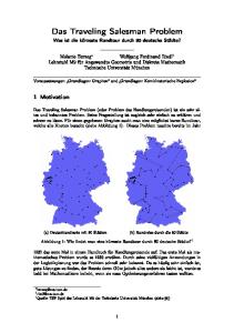
1. Introduction There have been a number of studies of human performance in the TSP (MacGregor & Ormerod, 1996; Graham, Joshi, & Pizlo, 2000; Vickers et al., 2001; Pizlo et al., 2006; Dry et al., 2006; Wiener, Ehbauer, & Mallot, 2009). These studies showed that human subjects can produce near-optimal tours very quickly. This performance generalizes to other combinatorial optimization problems like minimum spanning tree (MST) (Pizlo et al., 2005), shortest path (MacGregor, 2005), optimal stopping (Lee, 2005), or 15-puzzle (Pizlo & Li, 2005) (see Burns, Lee, & Vickers, 2006 for an overview). Optimization tasks are of importance not only in the context of human problem solving. Other cognitive functions like decision making, motor control, and perception can also be modeled as optimization tasks. It follows that using optimization tasks may be an effective way to study human cognition in general and problem solving in particular. The initial state in the TSP is usually a set of C cities laying on a 2D plane and the goal is to find the shortest tour of these cities (see an example of TSP and MST solutions in Figure 1 and the formal definition in Section 3). TSP belongs to the class of difficult optimization problems called NP-hard (Johnson & McGeoch, 1997). NP-hard means that in the worst case one may have to perform an exhaustive search in order to solve the problem. The number of all different tours in a C-city TSP is (C−1)! 2 , and thus grows very quickly with C, precluding exhaustive search. It is quite certain that human subjects do not search the whole or even substantial parts of the problem space when solving combinatorial optimization problems, because of memory and cognitive processing limitations. Many researchers have shown that humans produce close-to-optimal solutions to TSP in time that is (on average) proportional to the number of cities (Graham, Joshi, & Pizlo, 2000; MacGregor et al., 2000; Pizlo & Li, 2003). This level of performance cannot be reproduced by any of the standard approximating algorithms in computer science or operations research. Some approximating algorithms produce tours with lengths that are close to that of the shortest tour, but the time complexity is substantially higher than linear. Other algorithms are relatively fast but produce tours that are substantially longer than those produced by human subjects. Figure 1. Examples of combinatorial problems: TSP and MST.

A random instance of 25 cities

TSP tour

MST solution

The Journal of Problem Solving •

2D and 3D Traveling Salesman Problem

169

The TSP is usually defined as a problem on a 2D Euclidean plane. The positions of cities are known accurately and the distances between the cities are Euclidean distances.1 A problem solver faces a problem to determine the optimal (or nearly-optimal) tour. This is the usual experimental setup when human subjects were tested in previous studies (MacGregor & Ormerod, 1996; Graham, Joshi, & Pizlo, 2000; Vickers et al., 2001; Pizlo et al., 2006). The subject is shown the TSP problem on a computer screen, with the subject’s line of sight being orthogonal to the screen at the center of the screen (as shown in Figure 2). When the subject fixates his eye at the center of the screen, the retinal image in the subject’s eye is a scaled copy of the image on the computer screen. It follows that an optimal tour for the problem on the subject’s retina is also an optimal tour for the problem shown on the computer screen. Furthermore, a suboptimal tour with a relative error (ε) for the problem on the subject’s retina is a suboptimal tour with the same error for the problem on the computer screen (the relative error is defined as the difference between the length of the tour produced by the subject and the length of the optimal tour, normalized to the latter; see Section 3.3).

subject

computer screen

Figure 2. A typical experimental setting for testing human subjects in TSP, where the cities are presented on the computer screen.

This laboratory setting does not generalize to real-life situations. In real life, the cities are not necessarily restricted to a plane. Instead, they may reside on a 2D surface or in a 3D volume and their distances are almost never known accurately. Furthermore, the problem is likely to occupy a large part of the subject’s field of view, rather than the central 20 degrees, as in the case of experiments where the problems are shown on a computer screen. Consider the task of collecting tennis balls on a tennis court, the task tested in our Experiment 1 (see Section 4.1 and Figure 3). The TSP problem in this case occupies a large part of the subject’s field of view. In fact, once the subject is in the center of the problem space, some parts of the problem are outside of her visual field. She cannot see the whole problem at one glance. Furthermore, the subject cannot solve the 1 L2 norm.

• volume 3, no. 2 (Winter 2011)

170

Haxhimusa, Carpenter, Catrambone, Foldes, Stefanov, Arns, and Pizlo

problem on her retina because the retinal image is a perspective transformation of the original problem. In order to estimate the actual distances on the tennis court, the subject has to perform back-projection of the retinal image (i.e., reconstruct the positions of the tennis balls on the tennis court). Note that even small errors in this estimation will lead to large errors in the reconstructed distances on the floor. For example, assume that the actual slant is 80 degrees (as it was often the case in our experiment), and that the slant is underestimated by 1 degree (this magnitude of error is quite realistic considering the accuracy of the visual and vestibular system). This error in estimated slant of perspective projection would lead to 10% errors (tan(80 deg)/ tan(79 deg)) in estimating distances on the floor. We recently measured subjects’ ability to judge distances between objects in a real scene whose dimensions were 5 by 5 meters (Kwon et al., 2010). The resulting random errors in judging distances (5-8%) corresponded to the error in the estimated slant of the floor of about 1 degree. This means that our assumption about 10% errors is quite reasonable. Will these errors impact substantially the quality of the TSP tours? Not necessarily, considering the fact that even a large error in estimating individual distances may lead to only small errors in the length of a TSP tour. This issue will be discussed in some more detail after psychophysical results are presented. Figure 3. Presentation of cities on the tennis court. subject

10° ·

tennis court

This tennis court experiment was replicated in a virtual reality room (Purdue’s FLEX, a CAVE2-like device as shown in Figure 4). Using the FLEX it is quite easy to place simulated tennis balls on the simulated floor or in the 3D volume. The FLEX consists of four screens (three walls and the floor). The subject can move within the FLEX by walking. The head tracker records the position of the subject and updates the visual information, in order to adequately simulate the change of the visual scene. The subject wears goggles that provide her with binocular vision. The paper is structured as follows. After a short section on related works (Section 2), we formally define the problem (Section 3) and present psychophysical results (Section 4) and then the model (Section 5). We also fit the model to the subjects’ data. The paper ends with a conclusion section. 2  Cave Automatic Virtual Environment.

The Journal of Problem Solving •

2D and 3D Traveling Salesman Problem

171

Figure 4. Purdue’s FLEX virtual reality room. ceiling

wall wall

floor

2. Related Work The first study on human problem solving in TSP that used pyramid algorithms as models of the mental mechanisms was done by Graham and his colleagues (Graham, Joshi, & Pizlo, 2000; Pizlo, Joshi, & Graham, 1994). These authors modeled the mental mechanism involved in solving the visual version of the E-TSP. It has been shown (Graham, Joshi, & Pizlo, 2000; MacGregor et al., 2000) that subjects’ tours are, on average, only few percent longer than the shortest (optimal) tours, and the solution time was linearly related to the number of cities. Graham, Joshi, and Pizlo (2000) formulated a pyramid algorithm for E-TSP motivated by the failure to identify an existing algorithm that could provide a good fit to the subjects’ data. More recently, hierarchical algorithms have been used to model mental mechanisms involved in other types of visual problems (Pizlo & Li, 2003, 2004; Wiener, Ehbauer, & Mallot, 2009) (e.g., 15-puzzle problem, MST, etc.). The main aspects of the hierarchical models (Graham, Joshi, & Pizlo, 2000; Pizlo & Li, 2003; Pizlo et al., 2006; Haxhimusa et al., 2009) are: • multi-resolution pyramid architecture • a coarse-to-fine process of successive approximations to the solution All these models can be summarized as having two types of processes, bottom-up and top-down. The bottom-up processes in pyramids can be considered as building the problem representation, that is, understanding the problem (Newell & Simon, 1972). The solution to the problem is produced by a top-down, coarse-to-fine sequence of search

• volume 3, no. 2 (Winter 2011)

172

Haxhimusa, Carpenter, Catrambone, Foldes, Stefanov, Arns, and Pizlo

steps in the problem representation. Pyramid algorithms are suitable for problems such E-TSP since they solve (approximately) global optimization tasks without performing a global search. The computational complexity of these models is very low and similar to that characterizing mental processes (i.e., linear or close to linear). At the same time, the solutions produced by these models are characterized by similar errors as those produced by the subjects.

3. TSP 3.1. Notation T: set of cities

τ : tour of T l(τ): length of the tour τ τopt: optimal tour of T found by the optimal solver, and its length l(τopt) τpyr : solution of T by a pyramid model, and its length l(τpyr) τ*: intermediate solution of T, and its length l(τ*) 3.2. Definition of the TSP Let the cities of the TSP be represented by vertices (c ∈ C) of the input graph G and the intercity neighborhoods by edges (e ∈ N) (see Figure 5b). Each vertex of the input graph must have at least two edges for the TSP tour to exist. Moreover, the graph is attributed, G = (C, N, wv , we ), where we : N →R+ is a weighted function defined on edges N . The weights we are distances (e.g., Euclidean) in the TSP and wv : C → RN+ is a weighted function defined on cities C (e.g., each vertex [city] has as weights its position in the Cartesian coordinate system, thus N = 2 for 2D TSP and N = 3 for 3D TSP). The goal in TSP is to find a nonempty ordered sequence of vertices and edges (v0 , e1, v1, . . . , vk −1, ek , vk , . . . , v0 ) over all vertices of G such that all the edges and vertices are

Figure 5. 2D E-TSP, its graph representation and a TSP tour of a subject.

a) problem instance

b) graph G

Tour τ of subject ZL

The Journal of Problem Solving •

2D and 3D Traveling Salesman Problem

173

distinct, except the start and the end vertex v0 . This tour is called optimal tour τopt if its length l(τopt) defined as the sum of edge weights is minimal, that is,

( )

l  opt = ∑ w e → min, (1) e∈

where we is the weight of edge e. In this work we use Euclidean distances between cities as weights of the edges. In general, humans and approximation algorithms do not produce an optimal tour. Finding the global minimum of Equation 1 (the optimal tour) is a hard computational problem (Johnson & McGeoch, 1997). 3.3. Error Definition The error ε is computed as the ratio of the length of the tour produced by the model (l(τpyr)) or by the human subject (l(τh)) and the length of the optimal tour (l(τopt)):3

( ) ( )

 l τ pyr  εm =  − 1 ⋅ 100%, (2)  l τ opt   l (τ )  h εh =  − 1 ⋅ 100%. (3)  l τ opt 

( )

4. Psychophysical Experiments 4.1. Experiment 1: Real and Virtual 2D Floor 4.1.1. Method

The size of the area in a large hall within which the cities (tennis balls) were placed was 55 × 55 feet.4 The number of cities, which represents the problem size C, was 5, 10, 20,5 and 50 (10 randomly generated problems per problem size). The 50-city problems were used only in the virtual reality setting. Consider first the problems on the real floor with real tennis balls. First, we put labels on the floor producing a regular grid of 12 × 12, with step of 5 feet. Each point in this grid had coordinates (i, j ), i, j = 0, · · ·, 11. The color of the labels was similar to the color of the floor. As a result, the labels were visible only from a 3  In this paper we use Concorde algorithm as optimal solver. The implementation of this algorithm can be found at www.tsp.gatech.edu/concorde html. 4  Roughly 17 x 17 meters. 5  Exact problems are given in the Appendix.

• volume 3, no. 2 (Winter 2011)

174

Haxhimusa, Carpenter, Catrambone, Foldes, Stefanov, Arns, and Pizlo

very close distance so the subjects could not use them to plan their tour or to estimate distances from a larger distance. Before each trial, two experimenters placed the tennis balls at the points of the grid representing the city positions. This process took several minutes. During this period the subject looked away. At the beginning of each trial, the subject stood at the initial position at the midpoint of one of the sides (coordinates 5.5, 11) of the 55 × 55 square. When the trial started, the subject walked around the hall with a bag, collected the tennis balls, and returned to the starting city. The starting city, which was the closest city to the initial position, was marked with two tennis balls: one of the balls was collected at the beginning of the tour production and the other was collected at the end. Without the second tennis ball in the starting city location, the subject would not know where the end of the tour is. Without returning to the end, the problem would not have been equivalent to a TSP problem. Marking the start position with two tennis balls meant that the subject was told which ball is the start/end city. The decision about which city is the start/end of the tour has no effect on the optimal tour. Subjects seem to have preferences about where to start solving the problem. It was reasonable to assume that in this setup, the subject would start with the tennis ball that is close to the initial position. The tour chosen by the subject was recorded in two ways. One experimenter had a hard copy of the current problem and was drawing the tour as the subject collected the tennis balls. Another experimenter was videotaping the entire experiment. The order of problems was random and different for different subjects. The actual problems were generated randomly with two constraints. First, the city locations were restricted to the positions of the 12 × 12 grid. Second, from several hundred problems, we chose those whose optimal solutions changed maximally when the problems were compressed along the y-axis by a factor of 2. By doing this we were trying to select problems whose accurate solution required accurate perception of Euclidean distances on the floor. Recall that the subject’s retinal image is a perspective projection of the floor; we wanted to make sure that the subjects were solving the problems on the floor, rather than the problems on their retinal images. Six subjects were tested in the real TSP and five in virtual TSP (the following subjects were naive: TS, MB, OK, JS, ER, and RJ; two authors [LA and ZP] were tested in both). All subjects were tested with the same problems, but in a random order. The subject’s task was to collect the tennis balls in the order that produced as short a tour as possible. The same problems, involving the same city positions, were used in the virtual reality replication of the experiment. Considering the fact that the FLEX has horizontal dimensions of roughly 3 × 3 meters, small movements of the subject around the simulated tennis court could be executed by walking around the FLEX. Larger movements could be simulated by using a wand. The subject could also use the wand to rotate the scene around her. The subject produced the tour by collecting the tennis balls. As a result, in the case of the real floor, the subject could not undo a move or start over if she did

The Journal of Problem Solving •

2D and 3D Traveling Salesman Problem

175

not like the tour produced so far. A similar experiment, in which subjects solved TSP with 5 to 10 cities in a real room measuring 6 × 8 meters has recently been reported by Wiener, Ehbauer, and Mallot (2009). In that study, the 25 grid positions were explicitly given by cardboard boxes. These boxes provided quite reliable depth cues for estimating distances. As a result, the depth reconstruction part was probably easier, compared to our experiment. 4.1.2. Results and Discussion

Tour errors for the real and virtual settings along with standard errors of the mean are shown in Figures 6 and 7. Consider first the TSP on the real floor. Except for one subject (MB), who missed a ball in a few problems with 10 and 20 cities, the performance of all subjects was quite consistent and similar to the performance, reported in previous studies, where the problems were presented on a computer monitor. Large errors in the case of MB were caused by the fact that he started solving the TSP problems without looking around. As a result, when he was ready to finish a tour, and return to the starting city, he realized that there was one additional tennis ball (city) to collect. The subject was not allowed to “go back” and correct the tour because the visited cities were not there anymore (the visited tennis balls had already been collected). As a result, the subject’s tour was substantially longer than the optimal tour. This did not affect substantially the proportion of optimal solutions for this subject, but it did affect his average error. The proportion of optimal solutions (not shown on graphs) ranged from 60 to 90% for 5 cities, 50 to 80% for 10 cities, and 0 to 30% for 20 cities (recall that there were only 10 instances of a TSP for each problem size. As a result, the estimates of the proportions are not very reliable). These numbers are very close to the proportion of optimal solutions when the problems were presented on a computer screen (Pizlo et al., 2006). The average errors in the case of TSP on the real floor are also very close to the errors of solutions when the problems were presented on a computer monitor. In our study (Pizlo et al., 2006), the average errors of several subjects ranged between 0 and 1% for 10-city problems, between 1 and 4% for 20-city problems, and between 2 and 5% for 50-city problems. These results imply that the errors in reconstructing the actual distances from perspective images did not substantially (if at all) affect the quality of the solutions and, furthermore, that the subjects were able to integrate the visual information across the visual field. Apparently, accurate depth perception was not critical in solving TSP. In order to evaluate the effect of errors in reconstructing Euclidean distances on the floor, we performed a simulation experiment in which the Concorde and our pyramid algorithms solved TSP problems that were compressed along the y-axis by a factor corresponding to cos(α), where α ranged from 10 to 80 degrees. Compressing the problem by cos(α) corresponded to slanting the computer monitor relative to the line of sight by α. The error in the TSP solution (see Figure 8) was evaluated by comparing the order of

• volume 3, no. 2 (Winter 2011)

176

Haxhimusa, Carpenter, Catrambone, Foldes, Stefanov, Arns, and Pizlo

Figure 6. Human performance in 2D TSP.

a) Subjects’ performance in reality.

b) Subjects’ performance in VR.

cities in the solution of the compressed version of the problem to the order of cities in the optimal tour of the original version of the problem. It can be seen that the solutions are quite robust in the presence of compression of the problem. Compressing the y-axis by 13% (cos(30 deg)), which corresponds to errors in judging distances on the floor implied by a misestimation of the slant of the horizontal floor by about 1 degree (see our discussion of Figure 3 in Section 1), led to average errors in TSP solution of only about 1% for both the Concorde and our model. This is not completely surprising considering the fact that a TSP problem is solved for discrete set of cities. Namely, the order of cities in the solution, say, ABCD, will change to ACBD only if d(AB) + d(CD) > d(AC) + d(BD). If the rest of the tour stays the same, then the percentage error for the entire tour is likely to be much smaller than the percentage error in the two edges that were involved in changing the tour.

The Journal of Problem Solving •

2D and 3D Traveling Salesman Problem

177

Figure 7. Human and model performance in 2D TSP.

a) MST pyramid model’s performance with different values of parameter r.

b) Average performance of subjects and the performance of the MST pyramid model for r = 3.

There is also another interesting implication of the results shown in Figure 8. When a problem solver does not have access to accurate distances between pairs of cities, but only to approximate distances (which is a rule rather than exception in real life), there is almost no difference between the quality of solutions produced by an optimal TSP solver and those produced by our model. In the presence of errors in the data, all solutions are approximate. It follows that it is unnecessary to use an optimal TSP solver, whose computational complexity is exponential. One can use our model, whose complexity is linear with respect to the number of cities and which is able to produce essentially equivalent approximate solutions as the optimal solver. We could say, therefore, that when the data are not known exactly, there is no practical difference between P versus NP problems. The fundamental difference between these two classes of problems has primarily theoretical significance.

• volume 3, no. 2 (Winter 2011)

178

Haxhimusa, Carpenter, Catrambone, Foldes, Stefanov, Arns, and Pizlo

Figure 8. Mean and standard deviation of errors produced by an “optimal” algorithm (Concorde) and by our pyramid algorithm (BP) under different angle of projection α. Both solved slanted TSP problems, but their performance was evaluated by using the original (not slanted) versions. 20 City Problems Concorde MST Pyramid: r =7 50

% Error

40

30

20

10

0

10

20

30

40 50 60 Angle of projections

70

80

It is important to point out that performance of five out of six subjects in the case of real TSP problems was high despite the fact that they could not undo movements or start over. This is consistent with our observations from experiments where the TSP was solved on a computer monitor, namely, that such corrections are rarely made. Once the subject decides how the problem should be solved, the subject executes the plan. The global aspects are decided first, and local decisions about the tour are not likely to affect the global features of the path. Results in the virtual reality replication of this experiment are similar, although there was more variability both within and across subjects. Specifically, the proportion of optimal solutions ranged from 50 to 80% for 5 cities, 50 to 90% for 10 cities, and 0 to 20% for 20 cities. The average errors for individual subjects are shown in Figure 6b. The range of errors was slightly larger in virtual reality than in the real version of TSP. Specifically, the maximal average error was 3% for 5 cities, 4% for 10 cities, and 6% for 20 cities. These maximal errors are only slightly worse than those in the case of TSP on the real floor and TSP on a computer monitor. These results suggest that the virtual reality environment is a reasonable representation of the real environment. 4.2. Experiment 2: 3D TSP 4.2.1. Method

We tested human and model’s performance on 3D TSP, that is, TSP in which the cities are distributed in a volume. To the best of our knowledge, human subjects have never been

The Journal of Problem Solving •

2D and 3D Traveling Salesman Problem

179

tested with such problems. Results of this experiment have important implications for models of human performance. At this point, there are three such models. The first is the pyramid model described here, the second is the convex-hull model with cheapest insertion (MacGregor et al., 2000), and the third is the crossing avoidance (van Rooij, Stege, & Schactman, 2003). Only the pyramid model can generalize to 3D space. The convex-hull in 3D is not a tour, but a surface. Even if one determines all relevant edges connecting the neighboring points on this surface, it is still not clear in which order they should be visited to produce a tour. In other words, there is no natural way to walk around a surface like a sphere. It follows that there is no natural extension of the convex-hull model to 3D space. Crossing avoidance cannot be a useful strategy either, because a polygonal line connecting C cities in 3D space is very unlikely to produce self-intersection. If either of these two models was a plausible explanation of how humans solve TSP, the tours produced by humans, in the case of 3D TSP, should be comparable to random tours. Only a virtual 3D version of the TSP was used because it is difficult to place multiple points or objects in a real 3D space. Spheres with diameter of 15 centimeters were generated within a cube 3 × 2 × 3 meters in the FLEX virtual reality system at Purdue. The number of cities (problem size C ) was 6, 10, 20, and 50. There were 10 randomly generated TSP problems for each problem size. The viewing was binocular and the subjects were free to move. The subject used a 3D pointer to indicate the order in which the cities were visited. Once the city had been visited, it changed color. The tour produced so far was marked by a polygonal line. The subject could undo a move recursively. Six subjects were tested. All of them had extensive experience with virtual reality systems. Two subjects (RJ, RP) were naive. 4.2.2. Results and Discussion

Proportion of optimal solutions (not shown on graphs) ranged from 50 to 100% for 6 cities, and from 30 to 40% for 10 cities. Only one subject found an optimal solution for only one 20-city problem. None of the 50-city problems were solved optimally by any of the subjects. These numbers are systematically lower than those for the 2D TSP (see above). For example, for 10-city problems, the proportion of optimal solutions ranged from 60 to 90% in the case of problems shown on a computer monitor and from 50 to 80% in the case of real 2D TSP problems. Average solution errors of the five subjects tested on a 3D TSP are shown in Figure 9. Note that these errors are only slightly higher than those for 2D TSP in a virtual environment (errors of one subject, RJ, were substantially higher: 5% for 10-city problems, 10% for 20-city problems, and 25% for 50-city problems and are not shown in this figure). These results contrast with subjective reports of the subjects. Whereas 2D TSP appears natural and easy, 3D TSP appears very unnatural and difficult. The subjects reported that they had very little confidence in what they were doing in the case of 3D TSP and that they

• volume 3, no. 2 (Winter 2011)

180

Haxhimusa, Carpenter, Catrambone, Foldes, Stefanov, Arns, and Pizlo

Figure 9. Human performance in 3D TSP.

expected their tours to be no better than random tours. This was clearly not the case. For example, an average error of a randomly generated tour for 10-city TSP was 85%. In contrast, the average error of our subjects in the case of 10-city 3D TSP was less than 3%. The fact that 3D TSP appears unnatural is not surprising because it is unnatural. Human beings are used to solving 2D visual navigation tasks on surfaces, such as floors and ground. 3D visual navigation tasks (diving or flying) have not been common, if present at all, during the last 200,000 years of human evolution. Nevertheless, the visual (mental) mechanisms that are involved in solving 2D navigation tasks can be applied to 3D tasks as well. 4.3. Model Fitting What is the nature of the mental mechanisms involved? According to our computational model, human subjects solve TSP problems by means of: • hierarchical clustering • top-down process of coarse-to-fine approximations to the solution tour Our computational model is described in Section 5. It has been designed for 2D TSP problems. However, the fact that the model operates on graphs makes it suitable for 3D TSP problems as well. In other words, no modification was needed in order to apply the model to 3D problems. Will the model be able to account for human performance in 2D as well as in 3D problems? The model’s averaged errors for several values of r, which represents the extent of local search, are shown in Figures 7a and 10a. In Figures 7b and 10b human performance averaged across subjects is plotted together with performance of the model for r = 3, which is the value that provides the best fit to the subjects’ results. Consider first the fit in the case of 2D problems. The model’s performance is slightly but systematically better

The Journal of Problem Solving •

2D and 3D Traveling Salesman Problem

181

Figure 10. Human and model performance in 3D TSP.

a) MST pyramid model’s performance with different parameter r.

b) Average performance of subjects and the performance of the MST pyramid model for r = 3.

than that of the subjects. There are at least two sources of this difference. First, in the case of TSP on the real floor, there was one subject who produced substantially higher errors because he forgot about one tennis ball in several problems. This affected the average plotted in Figure 7b. Second, recall that the subjects had to visually reconstruct the distances on the floor before solving the problems. The model, on the other hand, was given positions and distances without any errors. Results of our simulation experiment shown in Figure 8 indicate that the effect of reconstruction errors would lead, on average, to a 1% increase in the solution errors. We can conclude, therefore, that if the effect of these two factors were eliminated, the model would have fitted the subjects’ data very well. Next, consider 3D problems. It can be seen that the model’s performance is quite close to that of the subjects. In particular, the model’s errors in the case of 3D TSP are systematically

• volume 3, no. 2 (Winter 2011)

182

Haxhimusa, Carpenter, Catrambone, Foldes, Stefanov, Arns, and Pizlo

larger than those in the case of 2D TSP. This result resembles the results of the subjects. What is different in the 3D case is that now the value of parameter r has substantial effect on the model’s performance. Apparently, in the 2D case, all of the “work” is being done by the clustering operation and the coarse-to-fine tour refinement, and the effect of local search is minimal. This is not true in the 3D case. Here, the extent of local search matters and cluster size of three seems to best fit the results of the subjects. The fact that local search is important in a 3D TSP seems reasonable—there is an additional dimension, compared to the 2D case, that has to be analyzed. For example, cities on the perimeter of a unit circle in 2D is a trivial TSP problem, whose solution is the order of cities along the perimeter, whereas cities on the surface of a unit sphere is far from a trivial problem. It is simply not clear how to produce an optimal tour on the surface of a sphere. Note that three points are always co-planar in a 3D space. The fact that the model with r = 3 provides best fit to the subjects’ data in 3D TSP suggests that the subjects are solving a 3D TSP by using piece-wise planar approximations. The important fact is that the same model can account quite well for the results of the subjects in 2D and 3D problems.

5. Pyramid Model Many combinatorial optimization problems have problem spaces that are extremely large, so much so that the states of these problems cannot all be represented at once in the human memory (the number of tours in a 17-city TSP is larger than the number of neurons in the human brain). It seems quite obvious, however, that an effective solution of a problem, a solution that is more sophisticated than that produced by random search, must somehow involve information about the whole problem. The only plausible approach in such cases is to use global but coarse information about the entire problem space and fine, detailed information only about the current state. In fact, the global versus local distinction is not sharp. Instead of two levels, one global and another local, a set of levels with systematically varying degree of locality and globality could be used. The pyramid representation fulfills these requirements. Our pyramid model uses local to global and global to local processes to find a good solution (τapp), approximating the E-TSP. The main idea is to use: • bottom-up process to create the problem representation and reduce the size of the input • top-down refinement (search) to find an (approximate) solution A pyramid representation (Figure 11a and b) consists of a set of layers, each layer involving a number of processors that are assumed to work simultaneously and, to a large extent, independently. Each processor has information about one part of the image, called its receptive field (RF). The bottom layer (layer 0) corresponds to the level of

The Journal of Problem Solving •

2D and 3D Traveling Salesman Problem

183

Figure 11. Multi-resolution pyramid. 1 λ λ

h a processor

2

1 λ

n

I

receptive fields

a) Pyramid concept

level 0 representation tree

reduction window

b) Discrete levels

receptors on the human retina. The number of processors in the second layer (layer 1) is smaller by a factor of λ —this factor is called a reduction ratio, and it is greater than 1. Specifically, one processor (a parent) receives input from λ children in the layer below. It follows that receptive fields on the second layer are larger by a factor of λ than those on the first layer. Similarly, the number of processors on the third layer is again smaller by a factor of λ , and so on, until the top layer is reached, where there is only one processor. Processors on higher layers receive only some information about the content of their receptive fields. The number of levels in the pyramid representation with the base size I is equal to logλ (| I |) (Figure 11). This implies that a regular pyramid representation is built in O[log(diameter(I))] parallel steps (Jolion & Rosenfeld, 1994). In our model, the TSP input is represented by graphs. A level (k) of the graph pyramid consists of a graph Gk . Moreover, each vertex in the graphs pyramid is attributed. 5.1. Irregular Graph Pyramid Model The TSP problem is recursively simplified in the process of hierarchical clustering. The centers of the clusters are used in lieu of the cities. Close to the top of the pyramid representation, the problem is trivial because it has only two or three cities. The solution of this trivial problem is then refined in a coarse-to-fine process of successive approximations. The main steps of the algorithm are shown in Algorithm 1 and discussed in more detail in Sections 5.1.1 and 5.1.2. 5.1.1. Bottom-up Simplification Using an MST Graph Pyramid

The most fundamental operation in producing hierarchical representation is hierarchical clustering. Points, features, and states in a problem can be clustered based on their similarities and proximities. Hierarchical clustering, and the resulting hierarchical representations, called pyramids, seem to be essential in perception and problem solving. Clustering is a task of finding “natural” groupings. The first question is how natural groupings are determined. In other words, what makes points in a cluster more like one another than points

• volume 3, no. 2 (Winter 2011)

184

Haxhimusa, Carpenter, Catrambone, Foldes, Stefanov, Arns, and Pizlo

Algorithm 1—Approximating E-TSP Solution with a Pyramid 1: partition the input space by preserving approximate location: create the input graph—G0 2: reduce number of cities bottom-up until the graph contains a couple of vertices: build the problem representation—Gk , 0 ≤ k ≤ h 3: find the first approximation of the TSP tour at the top of the pyramid—τa 4: refine solution top-down, until all cities at the base level are processed: find the approximate solution of the E-TSP—τapp .

in other clusters? This question leads to two other, more specific ones (Duda, Hart, & Stork, 2001): how to measure the similarity between points and features, and how to evaluate a partitioning of the points and features into clusters. Similarity (dissimilarity) measures are usually related to distances. When clusters are formed based on distances, it is natural to expect that the distances among points within a cluster are smaller than the distances among points in different clusters. But similarity could reflect some abstract properties that cannot be directly translated to distances. In such cases, clustering based on similarities may or may not reflect the relations among distances (Wilson & Keil, 1999). The simplest example of clustering is that in the spatial domain. Spatial clustering has been a subject of studies of spatial memory (McNamara, Hardy, & Hirtle, 1989) as well as human performance in solving TSP (Pizlo et al., 2006; Haxhimusa et al., 2007; Xiaohui & Schunn, 2007, 2006; Wiener, Ehbauer, & Mallot, 2009). Both groups of studies clearly imply that humans can perform clustering, but the underlying mechanisms remain unknown. Clustering techniques are used in the computer science community to solve TSP as well (Climer & Zhang, 2006). Hierarchical partitioning is one of the best known methods of clustering in a topdown direction (Duda, Hart, & Stork, 2001; Lance & Williams, 1967), while agglomerative clustering works in the bottom-up direction. MST can be used to perform the latter (Duda, Hart, & Stork, 2001). In Graham’s model (Graham, Joshi, & Pizlo, 2000), clusters are not explicitly represented. Instead, the centers of the clusters are used in the E-TSP solution process. The centers are modes (peaks) of the intensity distribution produced by blurring the image. To make clusters explicit Pizlo et al. (2006) used an adaptive model in which top-down partitioning of the plane along the axis of Cartesian system was used. In the work of Haxhimusa et al. (2007) the clusters were built adaptively in a bottom-up manner. The problem representation in these studies was represented by a hierarchical tree (see Figure 11). Similarly to the work of Haxhimusa et al. (2009), we use the greedy technique to

The Journal of Problem Solving •

2D and 3D Traveling Salesman Problem

185

create clusters of the cities; specifically, we are motivated by the MST Borůvka’s algorithm (Neštřil, Miklova, & Neštřilova, 2001), since it naturally creates hierarchical representations and is adapted to the input data. For a given graph G0 = (C, N, wv , we) the vertices are hierarchically grouped into trees, as given in Algorithm 2. The idea of Borůvka step is to perform greedy operations like in Prim’s algorithm (Prim, 1957), in parallel, over the entire graph. The trees (clusters) are not allowed to contain more than r ∈ N+ cities. If each tree contains at least two cities, the pyramid has a logarithmic height (Kropatsch et al., 2005) and it follows that the reduction factor λ is 2 ≤ λ ≤ r. An example of how Algorithm 2 builds the graph pyramid (all levels) is shown in Figure 12b. Each vertex finds the edge with the minimal weight (solid lines in Figure 12b 1-5 and Figure 13a). These edges create trees of no more than r (in the figure r = 3) cities. Note that some vertices do not have solid lines. They cannot be connected to other clusters because of the limit on the size of the cluster (r). The trees produced at this stage are then contracted to the parent vertices (shown in Figure 12b). Different levels of the pyramid are represented by different vertex colors and sizes. The parent vertices together with edges that are not part of the contraction (dotted lines shown in Figure 13a) are used to create the graph of the next level. The new parent vertex’s attribute can be the center of gravity of its child vertices, or the position of the vertex near the center of gravity. Note that by preserving the relations between the children and their parents, we create a hierarchical representation of the problem (red solid lines shown explicitly for the last two levels of the pyramid in Figure 13). The algorithm iterates until there are s vertices at the top of the pyramid, and since s is small a full search can be employed to find an optimal tour τa at the top layer quickly. Algorithm 2—E-TSP Problem Representation Reduction by an MST Graph Pyramid 1: Input: Attributed graph G0 = (C, N, wv , we ), and parameters r and s 2: k ← 0

3: repeat 4:   ∀vk ∈ Gk find the edge e’ ∈ Gk with minimum we incident into this vertex 5:   using e’ create trees T with no more than r vertices 6:   contract trees T into parent vertices vk + 1 7:   create graph Gk + 1 with vertices vk + 1 and edges ek ∈ Gk \ T

8:   attribute vertices in Gk + 1 9:   k ← k + 1

10: until there are s vertices in the graph Gk + 1. 11: Output: Graph pyramid—Gk , 0 ≤ k ≤ h.

• volume 3, no. 2 (Winter 2011)

186

Haxhimusa, Carpenter, Catrambone, Foldes, Stefanov, Arns, and Pizlo

Figure 12. Steps of MST-based pyramid algorithm for solving TSP. a) Input: Cities

b) Bottom-up simplification — creating the pyramid represen tation 1) level 0

2) level 1

3) level 2

4) level 3

5) top: level h

c) T op-down refinemen t of tours τ a sim ulating the human fovea - expansion of paren t t o its children initial tour τ a v1

1) refining v 1

2) refining v 2

3) refining v 3

3) refining v 4

v2 v3

v

v4

v τ a1

τ a2

τ a3

τ a4

...

d) Output: TSP tour τ app

5.1.2. Top-down Approximations of the Solution

The tour τa found at the level h of the graph pyramid is used as the first approximation of the TSP tour τapp . This tour is then refined using the pyramid representation already built (τa1, τa2 , . . . ). Similarly to Pizlo et al. (2006) we use the simplest refinement, the one-path refinement (Haxhimusa et al., 2009). The one-path refinement process starts by choosing (randomly) a vertex v in the tour τa (say vertex v1 in Figure 12c and Figure 13b). Using the parent-child relationship, this vertex is expanded into the sub-graph G’h–1 ⊂ G’h–1 from which it was created, that is, its receptive field in the next lower level (encircled vertices in Figure 13b). In this sub-graph a path between vertices (children) and non-refined vertices is found that makes the overall path τa1 the shortest one. For example, in Figure 12b and Figure 13b, the shortest tour τa1 is shown by a solid line and is found by choosing the shortest path between the start vertex v’ and the end vertex v’ (non-refined vertices) and going through all the vertices (children of v1) of the receptive field of v1, RF(v1). Since

The Journal of Problem Solving •

2D and 3D Traveling Salesman Problem

187

Figure 13. Graph pyramid representation and the first TSP tour approximation (from Figure 12). Gh

G h− 1 a) Tree representation Last two levels of the pyramid

v1

τa

v

τ a1

G h− 1 v

b) Refining v 1 First appro ximation τ a1 of τ a .

the number of vertices (children) in G’h cannot be larger than r (in Figure 12 example r = 3), a complete search is a reasonable approach to find the path with the smallest contribution in the overall length of the tour τa1. Note that the edges in τa1 are not necessarily the contracted edges during bottom-up construction. The refinement process then chooses one of the already expanded vertices in G’h–1, and expands it into its children at the next lower level Gh−2 , and the tour τa2 is computed. The process of tour refinement proceeds recursively until there are no more parent-children relationships, that is, vertices at the base of the pyramid (level 0) are reached. After arriving at the finest resolution, the process of refinement continues by taking a vertex in the next upper level in the same cluster, and expanding it to its children. Note that the process of vertex expansion toward the base level emulates the non-uniform resolution of the human retina. The tour is refined to the finest resolution in one part whereas other parts are left in their coarse resolution representation. The process converges when all vertices in the pyramid have been “visited.” 6 More formally the steps are depicted in Algorithm 3 and Procedure 1, following Haxhimusa et al. (2009). Other refinement approaches can be chosen as well (Haxhimusa et al., 2009). Note that any of the vertices can be chosen as the starting point for the solution process. Different starting points are likely to lead to different tours. The choice of the starting point may account, at least in part, for individual differences in human solutions. 5.2. Algorithm Complexity of the Pyramid Model The bottom-up process uses a model of simplification that is motivated by MST Borůvka’s algorithm. Using a fully connected graph to represent the input instance, it follows that the bottom-up simplification algorithm has at least O(|C |2) time complexity (Papadimitiou 6  A demo is given in http://spiderman.psych.purdue.edu/yll/fovea_pyramid_tsp_demo.php.

• volume 3, no. 2 (Winter 2011)

188

Haxhimusa, Carpenter, Catrambone, Foldes, Stefanov, Arns, and Pizlo

Algorithm 3—E-TSP Solution by an MST Graph Pyramid Representation 1: Input: Graph pyramid Gk , 0 ≤ k ≤ h and the tour τa 2: τapp ← τa

3: v ← random vertex of τapp 4: repeat

5:   refine(τapp , v) /* refine the path using the children of v. See Prc. 1 */ 6:   mark v as visited 7:   repeat 8:    if v has unvisited children then 9:    v ← first unvisited child of v in τapp /* given an orientation */

10:    else if v has unvisited siblings then

11:    v ← first unvisited sibling of v in τapp /* given an orientation */

12:    else if v has a parent, that is, v is not a vertex of the top level then 13:    v ← parent of v 14:    else

15:    v ←  16:    end if

17:   until (v not visited) V (v = ) 18: until v =  19: Output: Approximation E-TSP tour τapp .

Procedure 1—refine(τapp , v): refine a path τapp using the children of v 1: Input: Graph pyramid Gk , 0 ≤ k ≤ h, the tour τapp , and the vertex v. 2: (c1, . . . , cn) ← children of v /* vertices that have been contracted to v */ 3: if n > 0 /* v is not a vertex from the bottom level */ then

4:   vp , vs ← neighbors of v in τapp /* predecessor and successor of v */

5:   p1, . . . , pn ← argmin{length of path {vp , cp1, . . . , cpn , vs}} such that p1, . . . , pn   is a permutation of 1, . . . , n /* optimal order of new vertices in the tour */ 6:   replace path {vp , v, vs} in τapp with path {vp , cp1, . . . , cpn , vs} 7: end if 8: Output: refined TSP tour τapp .

The Journal of Problem Solving •

2D and 3D Traveling Salesman Problem

189

& Steiglitz, 1998). This time complexity of Borůvka’s algorithm can be reduced easily to O(|N| log |C|) if instead of the fully connected graph one uses a planar graph, for example, Delaunay triangulation.7 Note that the presented Algorithm 2 can be parallelized leading to complexity O(log |C|) with O((|C|+|N|)α(|N|, |C|)/ log(|C|)) processors (Cole, Klein, & Tarjan, 1996), where α(|N|, |C|) is the Ackermann-Péter function. The complexity of the top-down process depends on the choice of the parameter r. The number of levels of the pyramid depends on r and is h = logr (|C|); thus the overall 1 1 1 number of vertices in the pyramid is (1+ r + r2 + · · · + r h )|C| ≤ 2|C|. In our current implementation the search time within each cluster is done in constant time, O(1). Finding the best path within r cities in an exhaustive search is r!. Thus the overall time complexity of the top-down process is O(k|C|), where k is a small constant.8 The parameter r has to be chosen as a compromise between the quality of the tour produced and the amount of search performed. In our experiments r = 3 led to results similar to that produced by human subjects. Of course, theoretically one can use r = |C|, which would lead to the brute force algorithm. The number s ∈ N+ of vertices in the top level of the pyramid is chosen so that an optimal tour can be found easily (s = 3, or s = 4). Note that larger s means a shallower pyramid and larger graph at the top, which also means higher time complexity to find the optimal tour at the top level. Thus r and s are used to control the tradeoff between the speed and quality of solution.

6. Conclusion We performed two psychophysical experiments in which the subjects solved the TSP problems on a real and simulated floor, as well as in a 3D volume. The results showed that the subjects’ performance was quite similar to that on a computer monitor. These results were modeled by our new pyramid algorithm, in which hierarchical clustering was performed by building the MST. The same model was able to account for the psychophysical results in 2D and 3D spaces. This was possible because the model uses graph representations of the problems. As a result, the 2D and 3D problems are treated in the model in exactly the same way. This fact opens a possibility for using our MST pyramid model to other problems, which are not spatial. Specifically, most, if not all non-spatial problems, such as theorem proving, can be represented by graphs, with nodes representing concepts and edges representing relations. Once a graph is constructed for a given problem, it should be possible to build a graph pyramid and then plan a solution by solving the shortest path problem in a coarse-to-fine direction. In fact, this kind of global-to-local approach has been proposed by Lakatos (1976) as a typical way of proving theorems by mathematicians. 7 |C| is the number of vertices, and |N| is the number of edges. 8  The authors are thankful to Filip Pizlo for pointing this out.

• volume 3, no. 2 (Winter 2011)

Haxhimusa, Carpenter, Catrambone, Foldes, Stefanov, Arns, and Pizlo

190

7. Appendix: TSP Used in the Experiments Tables 1, 2, and 3 show the exact coordinates of the cities (tennis balls) that were placed in an area of 55 × 55 feet. These problems were used in the experiments on a real floor and replicated in virtual reality simulated floor (see Section 4.1 for more details). Each line in the table (Problem #) is a single problem. Coordinates are pairs of numbers i and j. The 0, 0 position was the top left position of the grid. Table 1. 5-city problems. Coordinates of the cities i, j

Problem # 1

2,1

8,0

6,6

4,10

9,9

2

2,4

8,6

6,8

7,10

6,11

3

2,0

1,1

8,1

6,3

6,7

4

1,2

9,1

3,7

0,9

6,11

5

7,0

11,0

9,3

0,8

9,11

6

1,1

11,0

8,4

6,6

6,10

7

2,0

9,2

7,6

8,10

3,11

8

7,1

10,0

8,4

1,10

10,11

9

0,3

6,2

2,6

9,6

2,8

10

6,1

11,0

8,6

10,8

6,11

Table 2. 10-city problems. Coordinates of the cities i, j

Problem # 1

4,0

2,3

7,3

11,3

0,4

7,4

4,7

7,7

2,11

7,11

2

2,0

4,0

9,0

4,3

7,4

4,7

1,8

9,9

4,10

9,11

3

4,0

6,0

2,2

9,2

7,4

3,7

0,8

6,8

2,11

8,11

4

6,0

10,0

11,0

11,2

9,6

8,7

1,9

11,10

8,11

9,11

5

0,1

3,1

9,1

4,2

3,4

6,6

7,6

1,9

8,9

6,11

6

2,0

6,1

9,1

8,4

7,6

8,6

7,7

4,11 10,11

7

11,0

0,1

3,1

6,1

4,2

3,3

7,6

4,10

8

7,2

1,4

10,3

1,6

9,6

3,8

10,7

9

7,0

6,1

11,1

7,4

9,4

8,8

3,9

10

3,0

10,0

4,1

2,3

2,6

6,7

2,10

11,11

7,10

8,11

2,10

6,11

9,10

3,11

10,11

3,11

7,11

9,11

11,8

The Journal of Problem Solving •

2D and 3D Traveling Salesman Problem

191

Table 3. 20 city problems. Coordinates of the cities i, j

Problem # 1

3,0 10,6

4,0 4,7

7,0 11,7

10,0 6,8

6,1 10,8

9,1 11,9

11,1 3,10

0,2 4,10

4,3 9,10

7,4 4,11

2

2,0 10,4

10,0 2,6

6,1 3,6

8,1 7,7

0,2 8,8

7,2 1,9

11,2 6,10

9,3 8,10

1,4 10,10

7,4 10,11

3

0,0 6,6

3,0 8,8

4,0 9,8

7,0 1,9

11,0 3,9

3,2 2,10

8,2 6,10

9,2 7,10

9,3 10,10

8,4 3,11

4

3,0 11,6

4,0 7,7

8,0 10,7

10,0 3,8

7,2 0,11

3,3 3,11

8,3 4,11

11,3 7,11

9,4 10,11

5

0,0 8,4

7,0 4,6

10,0 1,8

2,1 1,9

11,1 4,9

0,2 3,10

2,2 4,10

3,2 7,10

10,3 10,10

2,4 2,11

6

0,0 6,6

3,0 10,6

2,1 9,7

6,1 10,7

8,1 9,9

1,2 10,9

8,3 3,10

0,4 8,10

2,4 2,11

10,4 6,11

7

7,0 1,6

4,1 2,6

11,1 8,6

1,2 3,7

3,2 0,8

7,2 10,8

8,2 2,9

10,2 3,11

6,4 7,11

7,4 8,11

8

1,0 11,4

3,0 2,6

4,0 4,6

6,0 6,6

10,0 8,7

4,1 6,8

3,2 9,9

3,4 2,10

6,4 7,10

7,4 1,11

9

11,0 4,4

0,1 11,4

1,1 2,6

3,1 8,6

4,1 3,7

6,1 6,8

8,1 1,10

0,3 1,11

1,3 6,11

9,3 8,11

10

3,0 6,8

7,0 7,8

8,0 8,8

11,0 8,9

0,1 0,10

4,1 2,10

9,1 10,10

8,2 6,11

8,4 9,11

4,6 10,11

0,2 8,10

References Burns, N. R., Lee, M. D., & Vickers, D. (2006). Are individual differences in performance on perceptual and cognitive optimization problems determined by general intelligence? Journal of Problem Solving, 1, 5–19. Climer, S., & Zhang, W. (2006). Rearrangement clustering: Pitfalls, remedies, and applications. Journal of Machine Learning Research, 7, 919–943. Cole, R., Klein, P. N., & Tarjan, R. E. (1996). Finding minimum spanning forests in logarithmic time and linear work using random sampling. In Annual Association for Computer Machinery Symposium on Parallel Algorithms and Architectures (pp. 243–250). Dry, M., Lee, M. D., Vickers, D., & Hughes, P. (2006). Human performance on visually presented traveling salesperson problems with varying numbers of nodes. Journal of Problem Solving, 1, 5–19. Duda, R. O., Hart, P. E., & Stork, D. G. (2001). Pattern Classification. John Wiley & Sons. Graham, S. M., Joshi, A., & Pizlo, Z. (2000). The traveling salesman problem: A hierarchical model. Memory & Cognition, 28, 1191–1204.

• volume 3, no. 2 (Winter 2011)

192

Haxhimusa, Carpenter, Catrambone, Foldes, Stefanov, Arns, and Pizlo

Haxhimusa, Y., Kropatsch, W. G., Pizlo, Z., & Ion, A. (2009). Approximating TSP solution by MST based graph pyramid. Image and Vision Computing, 27, 887–896. Haxhimusa, Y., Kropatsch, W. G., Pizlo, Z., Ion, A., & Lehrbaum, A. (2007). Approximating TSP Solution by MST based Graph Pyramid. In F. Escolano & M. Vento (Eds.), Proceedings of the 6th International Workshop on Graph-based Representation for Pattern Recognition (pp. 295–306). Volume 4538 of Lecture Notes in Computer Science . Johnson, D. S., & McGeoch, L. A. (1997). The traveling salesman problem: A case study in local optimization. In E. H. L. Aarts & J. K. Lenstra (Eds.), Local Search in Combinatorial Optimization. (pp. 215–310). John Wiley and Sons. Jolion, J.-M., & Rosenfeld, A. (1994). A Pyramid Framework for Early Vision. Kluwer. Kropatsch, W. G., Haxhimusa, Y., Pizlo, Z., & Langs, G. (2005). Vision pyramids that do not grow too high. Pattern Recognition Letters, 26, 319–337. Kwon, T., Shi, Y., Sawada, T., Li, Y. F., Catrambone, J., Sebastian, S., & Pizlo, Z. (2010). Human recovery of the shape of a 3D scene. Annual Meeting of the Society for Mathematical Psychology, Portland, OR. Lakatos, I. (1976). Proofs and Refutations. Cambridge University Press. Lance, J., & Williams, W. (1967). A general theory of classificatory sorting strategies: I. Hierarchical systems. Computer Journal, 9, 373–380. Lee, M. (2005). A generative model of human performance on an optimal stopping problem. 1st International Workshop on Human Problem Solving, Purdue University (http://psych.purdue.edu/tsp/workshop/program.html). MacGregor, J. (2005). Solution performance and heuristics in closed and open versions of 2d Euclidean tsps. 1st International Workshop on Human Problem Solving, Purdue University (http://psych.purdue.edu/tsp/workshop/program.html). MacGregor, J., & Ormerod, T. (1996). Human performance on the traveling salesman problem. Perception & Psychophysics, 58, 527–539. MacGregor, J. N., Ormerod, T. C., & Chronicle, E. P. (2000). A model of human performance on the traveling salesperson problem. Memory & Cognition, 28, 1183–1190. McNamara, T. P., Hardy, J. K., & Hirtle, S. C. (1989). Subjective hierarchies in spatial memory. Journal of Experimental Psychology: Learning, Memory & Cognition, 15, 211–227. Neštřil, J., Miklova, E., & Neštřilova, H. (2001). Otakar Borůvka on minimal spanning tree problem translation of both the 1926 papers, comments, history. Discrete Mathematics, 233, 3–36. Newell, A., & Simon, H. A. (1972). Human Problem Solving. Prentice Hall. Papadimitiou, C. H., & Steiglitz, K. (1998). Combinatorial Optimization: Algorithms and Complexity. Dover Publications Inc. Pizlo, Z., Joshi, A., & Graham, S. M. (1994). Problem solving in human beings and computers. Technical Report CSD TR 94-075 Department of Computer Sciences, Purdue University.

The Journal of Problem Solving •

2D and 3D Traveling Salesman Problem

193

Pizlo, Z., & Li, Z. (2003). Pyramid algorithms as models of human cognition. Proceedings of SPIE-IS&T Electronic Imaging, Computational Imaging (pp. 1–12). SPIE. Pizlo, Z., & Li, Z. (2004). Graph pyramids as models of human problem solving. Proceedings of SPIE-IS&T Electronic Imaging, Computational Imaging (pp. 205–215). SPIE. Pizlo, Z., & Li, Z. (2005). Solving combinatorial problems: The 15 puzzle problem. Memory & Cognition, 33, 1069–1084. Pizlo, Z., Stefanov, E., Saalweachter, J., Haxhimusa, Y., & Kropatsch, K. (2005). Adaptive pyramid model for the traveling salesman problem. 1st International Workshop on Human Problem Solving, Purdue University (http://psych.purdue.edu/tsp/workshop/ program.html). Pizlo, Z., Stefanov, E., Saalweachter, J., Li, Z., Haxhimusa, Y., & Kropatsch, W. G. (2006). Traveling salesman problem: A foveating model. Journal of Problem Solving, 1, 83–101. Prim, R. C. (1957). Shortest connection networks and some generalizations. The Bell System Technical Journal, 36, 1389–1401. van Rooij, I., Stege, U., & Schactman, A. (2003). Convex hull and tour crossings in the Euclidean traveling salesperson problem: Implications for human performance studies. Memory & Cognition, 31, 215–220. Vickers, D., Butavicius, M., Lee, M., & Medvedev, A. (2001). Human performance on visually presented traveling salesman problems. Psychological Research, 65, 34–45. Wiener, J. M., Ehbauer, N. N.,, & Mallot, H. (2009). Planning paths to multiple targets: Memory involvement and planning heuristics in spatial problem solving. Psychological Research, 77, 644–658. Wilson, R. A., & Keil, F. C. (1999). The MIT Encyclopedia of the Cognitive Sciences. MIT Press. Xiaohui, K., & Schunn, C. D. (2006). Global vs. local information processing in problem solving: A study of the traveling salesman problem. 7th International Conference on Cognitive Modeling.

Xiaohui, K., & Schunn, C. D. (2007). Global vs. local information processing in visual/spatial problem solving: The case of traveling salesman problem. Journal of Cognitive Systems Research, 8, 192–207.

Acknowledgment The authors were supported by the ASFOR. Y.H. was also partially supported by FWFP20134-N13 and FWF-S9103-N04.

Paper submitted: Aug 31, 2009 Paper accepted: September 23, 2010

• volume 3, no. 2 (Winter 2011)