© 2003-Present Jeeshim & KUCC625 (5/5/2005)
STATA Data Manipulation: Basics and Applications 7
1. Introduction 1.1 Dataset: Observations and Variables This section discusses data structure of a dataset with respect to observations and variables. 1.1.1 Data Structure of a Dataset A dataset is a data table that has a set of observations. An observation, often called case, is a collection of information of a unit of analysis. Individual information on the attributes of a unit of analysis is stored in a variable.1 Imagine a worksheet in Excel that arranged by row (observation) and column (variable). Figure 1.1 illustrates how a dataset looks like. The left visualizes concepts of observations and variables. The right shows a part of an actual STATA dataset. Figure 1.1 Observations and Variables in a Dataset +-------------------------------------+ var1 var2 ⋅ ⋅ ⋅ vark ⎧ | id age0 age male interest | |-------------------------------------| ⎪ obs { ⋅ ⋅ ⋅⋅⋅ ⋅ 1 | 1025 29 1 0 1.00 | ⎪⎪ | 1026 40 3 1 3.50 | Dataset ⎨ obs2 { ⋅ ⋅ ⋅⋅⋅ ⋅ | 1027 27 1 0 . | ⎪ ⋅ ⋅ ⋅ ⋅ ⋅ ⋅{ | 1028 34 2 . 5.00 | ⋅⋅⋅ ⋅⋅⋅ ⋅⋅⋅ ⋅⋅⋅ | 1029 35 2 1 4.00 | ⎪ … … … … … … … ⎪⎩ obsn { ⋅ ⋅ ⋅ ⋅ | 1226 50 4 1 3.25 | It is highly recommended to have unique identification in a dataset in order to trace observations back and forth. 1.1.2 Rules of Naming It is important to have proper names of files, variables, macros, functions, and labels in data analysis. In particular, variable name is most critical since data analyses are based on variables. • • • • •
Use characters (a- z and A-Z), numbers (0-9), or underscore (_) only.2 Begin with a letter.3 The shorter, the better. Do not exceed 10 characters unless necessary.4 Avoid reserved words or keywords (e.g., command and function). Use meaningful names associated with contents of the variable.
1
Observation is also called record or entity, while variable may be called field or attribute. Do not use special characters such as -, space, ~, !, @, #, $, %, ^, &, *, (, ), {, }, [, ], , ?, and /. 3 It is because underscore is often used in system variables such as _N, _n, _pi, _b, _coef, and _cons. 4 STATA allows up to 32 characters as a variable name. 2
http://www.masil.org
http://www.hangjung.org
© 2003-Present Jeeshim & KUCC625 (5/5/2005)
• • • •
STATA Data Manipulation: Basics and Applications 8
Make it consistent and systematic.5 Use lower cases unless necessary or required. Use underscore instead of space Use a value of the dummy variable.
1.1.3 Good and Bad Names Most common mistakes in naming are allowing blank (e.g., US citizen), beginning with a number (e.g., 2002_sale), and using a very long name (e.g., How_would_you_…). Table 1.1 compares good and bad examples of variable names. Table 1.1 Good and Bad Variable Names Good Example Bad Example gnp2002 real_int score1; gnp2003 reg_out; glm1 invest; interest male; black score1; score2;… citizen income; intUS03
Description
gnp-2002; gnp#2002 real interest rate 1st_score; 2003gnp REG; glm; ttest xxx; yyy; zmdje; gender; race math; math_1; math02 Are_you_a_US_citizen? INCOME; Int_us2003;
Avoid special characters Use underscore Begin with a character Avoid reserved words Use meaningful names Use a value of dummy Consistent and systematic The shorter, the better Use lower cases
Naming is a beginning point of data analyses. Bad naming may frequently bother you during the analyses. 1.2 STATA Basics STATA is available in a variety of platforms and flavors. STATA runs under UNIX, LINUX, Microsoft Windows and Apple Macintosh OS. 1.2.1 Three Flavors Stata has three different flavors. Stata/SE (Special Edition) is most powerful in that it can handle large data sets and matrices in a fast and safe manner. Intercooled Stata, a standard version, provides moderate capacity for ordinary users. Small Stata, a limited edition, is not available in UNIX machines. Table 1.1 summarizes major differences among the three flavors. This book mainly focuses on STATA/SE (release 8 and 9) under Microsoft Windows. Table 1.2 STATA Three Flavors Maximum Special Edition Observations Variables Dataset Width 5
Limited by memory 32,766 393,192
Intercooled Stata
Small Stata
Limited by memory 2,047 24,564
1,000 99 200
You can benefit from using array and wild card as in score1-score10, score??, vote*.
http://www.masil.org
http://www.hangjung.org
© 2003-Present Jeeshim & KUCC625 (5/5/2005)
Command Macro String Variable Matrices One-way Table Two-way Table
1,081,527 characters 1,081,511 characters 244 characters 11,000 by 11,000 12,000 12,000 by 80
STATA Data Manipulation: Basics and Applications 9
67,800 characters 67,784 characters 80 characters 800 by 800 3,000 300 by 20
8,697 characters 8,681 characters 80 characters 40 by 40 500 160 by 20
STATA puts a dataset into computer memory (including virtual memory), but it does not automatically use all the memory available in your computer. STATA/SE by default assigns 10MB for dataset. When reading a large dataset, you may need to adjust memory size, maximum number of variable, and/or matrix size using the .set memory, .set maxvar, and .set matsize commands.6 . set memory 150m, permanently . set maxvar 10000 . set matsize 2000
You may also use virtual memory to have enough room for a dataset at the expense of processing speed. . set virtual on
1.2.2 Variable Types STATA supports six variables types, which are grouped into real number, integer, and string. Default type is float, single precision real number. Date type is deal with the string type and conversion functions. Table 1.3 STATA Variable Types Keyword Type Bytes Format Range float double byte int long str#
Real Real Integer Integer Integer String
4 8 1 2 4 #
%9.0g %10.0g %8.0g %8.0g %12.0g -
1.70141173319×(-1038 ~1036) (8.5 digits of precision) 8.9884656743×(10307~10308) (16.5 digits of precision) -127 ~ 100 -32,767 ~ 32,740 -2,147,483,647 ~ 2,147,483,620 str1 through str244*
You need to use proper variable types in order for efficient memory management. For instance, the byte type (1 byte) is best for five-point Likert scale. Use int (2 bytes) rather than long (4 bytes), and float (4 bytes) rather than double (8 bytes), unless required. 1.2.3 Default Extensions Table 1.4 summarizes default extensions used in STATA. These default extensions are often omitted. 6
However, increasing memory size does not always improve the overall performance of STATA. The optimal memory size depends upon computing resources and the size of the dataset.
http://www.masil.org
http://www.hangjung.org
© 2003-Present Jeeshim & KUCC625 (5/5/2005)
Table 1.4 STATA Default Extensions Default File Types .dta .do .ado .log .smcl .raw .out .dct .gph
STATA format dataset STATA do-file Automatically loaded do-file Log file in the text format Log file in the SMCL format ASCII text file Files saved by the .outsheet ASCII data dictionary Graph image
STATA Data Manipulation: Basics and Applications 10
Related Commands .use and .save .do and .doedit .doedit .log .cmdlog .infile, .infix, and .insheet .outsheet .infix .graph
1.2.4 Length of Names and Labels Table 1.5 summarizes the maximum length of names and labels. Table 1.5 Length of Names and Labels Keyword Maximum Length Variable Name 32 characters String Variable 244 characters Dataset Label 80 characters Variable Label 80 characters Value Label Name 32 characters Value Label 32,000 characters* Language Label Local Macro Name 31 characters Global Macro Name 32 characters Macro Variable 1,081,511 characters * The intercooled allows only 80 characters.
Notes Function name? .label data “…” .label variable var_name “… ” .label define lbl_name # “…”; .label values var_name lbl_name .label language lang_name .local mac_name “…” .global mac_name “…”
1.3 STATA Interface There are three ways to communicate with STATA: Interactive mode, non-interactive mode, and point-and-click. 1.3.1 Interactive mode STATA is a command-driven application. This interactive mode enables users to communicate with STATA step by step. Users need to type in a command and hit ENTER to run the command. Then, STATA interprets the command, processes the job, and return its result to users (Figure 1.1). Figure 1.2 STATA’s Interactive Mode
http://www.masil.org
http://www.hangjung.org
© 2003-Present Jeeshim & KUCC625 (5/5/2005)
STATA Data Manipulation: Basics and Applications 11
STATA systematic grammar structure and abbreviation rules makes it efficient and flexible to perform many simple tasks. STATA must come in pretty handy. Unlike compilers, STATA command interpreter keeps analysis results in memory even after executing commands so that users can conduct necessary follow-up analyses without running entire analyses again. 1.3.2 Non-interactive mode (batch mode) The non-interactive mode executes a set of commands written in a text file. Classical statistical software like SAS uses this mode of communication. Instead of running individual commands one by one in the interactive mode, users may write a .do file, a batch file, in which a set of commands are organized. Writing a do file is efficient especially when a bundle of commands needs to be repeated many times.7 In order to open the STATA Do-file editor, click WindowÆDo-file Editor or pressing Ctrl+8. Alternatively, run the .doedit command or click the Do-file editor icon may also use a text editor like Notepad to write a do file.
. You
Figure 1.3 STATA’s Do-file Editor
Once a .do file is ready, you may execute the batch job by running the .do command in the command window. Alternatively, you may choose ToolsÆDo menu (Ctrl+D) or click
7
Another type of programs is the .ado file. In fact, many STATA commands are based on .ado files. Although StataCorp provides basic .ado files, users also can write their own .ado programs to add their own commands to STATA. The .do files include typical STATA commands, while .ado programs need to be written in the STATA ado language. This book does not address .ado programming.
http://www.masil.org
http://www.hangjung.org
© 2003-Present Jeeshim & KUCC625 (5/5/2005)
STATA Data Manipulation: Basics and Applications 12
in the Do-file Editor window. When you wish to execute only a part of commands, highlight the block of commands using a mouse, and choose ToolsÆDo Selection menu. 1.3.3 Point-and-Click (Graphical User Interface) STATA’s point-and-click provides graphic user interface environment, where users pull down menus and select a proper menu of a command to invoke the dialog box. STATA echoes the command on the basis of information provided in dialog boxes. In order to invoke a proper dialog box, run the .db command or use shortcuts. For instance, you may run .db save command or press Ctrl+S (pressing S key while the Ctrl key is pressed), which is equivalent to clicking FILEÆSave. 1.4 STATA Commands 1.4.1 Command Conventions There are several conventions for STATA commands. • • • • • •
Commands are lowercased. Commands, variable names, and options can be abbreviated. No character is required at the end of a command. A command and its options should be separated by a comma. There is no comma between variables and between options. A dependent variable precedes a set of independent variables.
1.4.2 Abbreviations STATA commands, variable names, and options can be abbreviated to the shortest string of characters as long as they are uniquely identified. The minimum abbreviations are underlined in help and manuals (e.g., tabulate). However, some commands like the .replace cannot be abbreviated. Users also use wildcards such as ?, *, and ~ when abbreviating variable names (see Table 1.5). 1.4.3 Command Structure A STATA command in general consists of, • • • •
A command (with subcommands) A list of variables (dependent and independent variable) Qualifiers (in and/or if) Option(s)
http://www.masil.org
http://www.hangjung.org
© 2003-Present Jeeshim & KUCC625 (5/5/2005)
STATA Data Manipulation: Basics and Applications 13
A command may or may not have their subcommands. A command may have a series of options as follows. . list state lung cigar, nolabel noobs separator(10)
1.4.4 Listing Variables You may list all variables to be used. Omitting a list of variables implies all variables in a dataset. STATA allows various ways of listing variables using wildcards (Table 1.5). Table 1.6. Wildcards Wildcards Descriptions ? * ~ -
Any character Any characters zero or more characters Specifying range of variables
Examples d? re* mil~um gender-rank
For example, d? means the variables beginning with d and ending with any single character and number (e.g., da, db, dc… d1, d2, d3…), while re* indicates any variables beginning with re (e.g., retain and return). The in~t means any variables beginning with in and ending with t. (e.g., invent and interest ) The gender-rank indicates all variables from gender through rank of the variable list in a dataset. Followings are some examples of using wildcards in listing variables. . list . list state d? re* . list state-lung in~t
The in and if qualifiers specify a subset of a dataset to which a command is applied. 1.4.5 Selecting Observations The if and in qualifiers specify a subset of a dataset to which a command is applied. The if qualifier selects observations that meet the conditions imposed. You may use & (and) and/or | (or) relational operators to provide more than one condition. . list if area==3 . list state cigar lung if (area==4) & (lung >= 10)
The in qualifier directly specifies the range of observations. You may use observation numbers (record numbers) or some symbols indicating particular observations (Table 1.6). Note the “/” separates beginning and ending observation numbers. . . . .
list in 10 list in 10/50 list cigar-kidney in f/10 sum bladder cigar in f/l
Table 1.7 Symbols of the in Qualifier. http://www.masil.org
http://www.hangjung.org
© 2003-Present Jeeshim & KUCC625 (5/5/2005)
STATA Data Manipulation: Basics and Applications 14
Symbols
Example
Meaning
# -# 1 (or f) -1 (or l)
in in in in
The 10th observation The 10th observation from the last From the first observation through the 10th From the 15th observation through the last
10 -10 1/10; in f/10 15/-1; in 15/l
However, you may not list more than one observation numbers without the / operator, nor specify observation numbers as well as the range of observations at the same time. 1.5 Commands, Function, and Operators 1.5.1 Basic Commands Table 1.8 summarizes the basic commands frequently used in STATA. Table 1.8 Commands .display .use, .save .describe .summarize .tabulate .list .edit, .browse .generate, .egen .replace, .recode .count .version .memory, .set memory .format .lookfor .quietly, .noisily
Description Echo strings and values of scalar expressions Load and save a dataset Describe dataset in memory Summary statistics One-way and two-way table of frequencies List values of variables Edit and view a dataset in Data Editor Generate variables Modify and recode variables Count the number of observations Return release number and set the command interpreter Check and set memory size Specify variable display format Search for sting in variable names and labels Suppresses and turns back STATA output
1.5.2 Operating System Commands Table 1.9 summarizes useful operating system commands. Note that the .pwd and .rm are available only under Macintosh OS and UNIX, respectively. Table 1.9 STATA Operating System Commands Command s Descriptions .cd (.pwd in Mac OS) .copy .dir (or ls) .erase (.rm in UNIX) .mkdir .shell .type
Change a directory Copy files List directories and files Remove files Create a directory Invoke operating system temporarily View contents of a text file
1.5.3 Operators and Symbols http://www.masil.org
http://www.hangjung.org
© 2003-Present Jeeshim & KUCC625 (5/5/2005)
STATA Data Manipulation: Basics and Applications 15
Table 1.10 illustrates various operators used in STATA. Note that the equal operator is not “=” (assignment), but “==.” Table 1.10 STATA Operators Types Operators Arithmetic Operator Relational Operator Logical Operator Assignment Concatenation Backward Shift
+, -, *, /, ^ (power) >, >=, area = 2 Variable | Obs Mean Std. Dev. Min Max -------------+-------------------------------------------------------cigar | 12 23.70667 2.762431 19.96 27.91 lung | 12 18.31667 3.68153 12.12 22.8 ...
1.6.2 The .by Command The .by command with the sort option is equivalent to the .bysort.
http://www.masil.org
http://www.hangjung.org
© 2003-Present Jeeshim & KUCC625 (5/5/2005)
STATA Data Manipulation: Basics and Applications 17
. by area, sort: sum cigar lung
Alternatively, you may omit the sort (or s) option, if you sort the variable in advance. . sort area . by area: sum cigar lung
1.7 Using the .display Command The .display (or .di) command displays strings and values of various scalar expressions. This command also echoes outputs of a program. 1.7.1 Displaying Strings and Values of Variables The following is an example of displaying a string and values of system variables. Note that the _pi below is a system variable. . display “Pi is “ _pi Pi is 3.1415927
Next example displays values of two variables using explicit subscripts. The number in a bracket indicates the observation number (record pointer). . display state[12] cigar[12]
1.7.2 Using As a Hand Calculator This command enables users to use STATA as a calculator. The followings show how various expressions can be used in this command. . display 5*5*3.14 . display (1.3)^(1/12)-1 . di (6.4-5.0)/sqrt(10)
1.7.3 Using Probability Distributions One of the biggest benefits of the .display command is that users can get p-values without referring probability distribution tables. The various probability distribution functions are used in the expressions of this command (Table 1.14). Consider the following examples. . di normal(1.96) . di (1-normal(1.96))*2
The .normal(z) returns the cumulative probability of the standard normal distribution. So the second command gives you the two-tailed p-value of the z score 1.96.
http://www.masil.org
http://www.hangjung.org
© 2003-Present Jeeshim & KUCC625 (5/5/2005)
STATA Data Manipulation: Basics and Applications 18
The ttail(df , t) returns the reverse cumulative (upper-tail only) Student’s t distribution. The first example below returns the two-tailed p-value of the t value 2.086 with degree of freedom 20. . disp ttail(20, 2.086)*2
The chi2tail(df, c) gives you the reverse (upper-tail) cumulative probability of the chisquared distribution. Similarly, the Ftail(df1, df2, F) returns reverse (upper-tail) cumulative probability of the F distribution. Note that the F is uppercased and that the first number is the degree of freedom for numerator. . disp chi2tail(10, 18.307) . disp Ftail(5, 10, 3.325)
The t, chi-squared, and F scores used above, in fact, are critical values of the distribution at the .05 level. Thus, all examples produce .05. Table 1.14 Major Probability Distribution Functions Functions Descriptions binomial(n, k, p) binormal(h, k, p) chi2(d, x) chi2tail(d, x) F(d1, d2, f) Fden(d1, d2, f) Ftail(d1, d2, f) normal(z) normalden(z) normalden(z, s) tden(d, t) ttail(d, t)
http://www.masil.org
Binomial probability distribution of k or more successes in n trials Joint cumulative distribution of bivariate normal Cumulative chi-squared distribution Reverse cumulative (upper-tail) chi-squared distribution Cumulative F distribution Probability density function of the F distribution Reverse cumulative (upper-tail) F distribution Cumulative standard normal distribution Standard normal density Rescaled standard normal density Probability density function of Student’s t distribution Reverse cumulative (upper-tail) Student’s t distribution
http://www.hangjung.org