Proceedings of the International Commission on History of Meteorology 1.1 (2004)
11. Data Collection and the Ozone Hole: Too much of a good thing?1 Maureen Christie Department of History & Philosophy of Science University of Melbourne, Australia
The Problem It was 1985. An article had just appeared in Nature announcing a large seasonal disappearance of ozone from the atmosphere over the Antarctic2. The community of atmospheric scientists was in disarray. Why? What was going on? Science in the late twentieth century appears to be a large-scale, orderly, and conservative enterprise. Major surprises were rare, but they did occur from time to time. Why was this announcement such a surprise? Everyone was focussed on the ozone layer and possible human influences. There had been both scientific and public debate for a decade. 1.
Scientists had been strenuously searching for ozone depletion. Their best current data indicated a possible depletion of 2-3 % — barely detectible. But this article claimed local depletions of up to 60%.
2. Why did the data come from a single British ground observing station? NASA had a satellite in orbit, continuously monitoring ozone levels world-wide. The
Data Collection and the Ozone Hole
100
British team leader was a good scientist, with a reputation for careful, conservative, and scholarly work. But he was not widely known as a leading atmospheric scientist. Those atmospheric scientists who knew Farman knew he would not lightly publish such an article; many did not know him. 3. A major new research effort had been put into investigations of stratospheric circulation and chemistry. Better understandings of chemical mechanism and atmospheric circulation, along with improvements in computer technology had been incorporated into the modelling. None of the models had indicated anything unusual happening in the Antarctic. Stratospheric reaction systems are largely light-driven. Everyone was expecting daytime in the upper tropical stratosphere as the likely place for active chemistry. Polar air in the lower stratosphere is second only to night-time for absence of ultraviolet light! It was regarded largely as a chemically inert reservoir. 4. The article shows an anomaly only in the Antarctic, only in the spring months, and only in years since 1977. A depletion that is both local and seasonal, and started quite suddenly in 1976 or 1977 was a surprise. 5. In the context of great scientific interest in stratospheric ozone, why did it take eight years for the announcement to be published? Four years of data collection — up to1980 — would have been enough to confirm that there was a persistent trend rather than just an anomalous season or two. The same four years could have been used for instrument calibration and re-checking, to rule out artefactual explanations. Why did the article not appear in 1981? These issues, then, provide the focus of this article. Several important questions arise: ♦ Why did the publication take so long when everyone was looking so hard? ♦ Why had the announcement not come from the NASA satellite team, which was better resourced, and had been engaged in more intensive data collection? ♦ Why was the announcement made on the basis of data from a single ground station? There were over 200 such stations around the world, 17 of them in the Antarctic. I will address these questions in reverse order.
Other Ground Stations A large network of ground stations for worldwide ozone monitoring was set up for the International Geophysical Year 1957-1958. But the initial enthusiasm waned. Funding for personnel and instrument maintenance and calibration fell away in many cases. Some stations were reporting ozone readings on an intermittent and irregular basis. Some had stopped and restarted at various stages. Some gave up altogether. When ozone depletion became an issue in the early 1970s, new stations joined the network, and some dormant programmes were resurrected.
Proc. ICHM 1.1 (2004)
101
Most of the monitoring stations classified as Antarctic are located near or outside the Antarctic Circle. They did not fall within the area affected by the phenomenon, or at least did not consistently do so. From one of these stations, the Japanese Syowa station, there is a conference report from 1984 of anomalously low ozone in the 1983 Austral spring season3. It was presented at the time as a singular rather than an ongoing phenomenon. There are few remaining stations. The French station at Dumont d'Urville was then in a dormant phase, at least as far as reporting ozone readings is concerned. Soviet operations at Mirnyy had been hampered from the start with appalling weather conditions, and they were in the process of relocating most of their Antarctic operations to a more amenable location at Molodezhnaya. Observations from Mirnyy were both sparse and questionably erratic. The ozone monitoring instrument at the American base at the South pole had its own particular problem at the crucial time. That left only the British station at Halley Bay to make the crucial observations.
The Satellite Observations The satellite programme collected about 140,000 readings per day, covering the whole surface of the Earth. Computing technology was primitive by today’s standards. The readings were analysed for quality control purposes, and archived on magnetic tape for distribution to scientists interested in working with the data. Local averaging and graphical presentation were not then within the scope of the software. The ozone maps that we are now familiar with were still some years away. There is a nice myth with an appropriate moral, which has been widely circulated to explain the failure of the satellite team to discover the Antarctic Ozone Hole. One of several published sources puts it in these terms: Interestingly, it was discovered that US measuring satellites had not previously signaled the critical trend because their computers had been programmed automatically to reject ozone losses of this magnitude as anomalies far beyond the error range of existing predictive models.4 The moral, of course, is to beware of automatic routines, and to be very careful about what you do with outliers. This story is at best a gross over-simplification, and more probably just plain wrong! Within a year after the publication of the British Antarctic Survey paper, an article by the NASA scientists appeared in Nature5. It confirms the British data, and clarifies that the phenomenon covers most of the Antarctic continent, and not just the Halley Bay area. No hint of an excuse or explanation is given for the late appearance of their article. But it is clear that computer programs had not ‘rejected’ anomalously low ozone readings, else they could not have been resurrected for analysis in this article. At the very least, the satellite data had been properly archived! An account provided by one of the NASA scientists is published elsewhere6. Anomalouly low ozone levels were not rejected, but flagged. Early in 1984, the quality
Data Collection and the Ozone Hole
102
control team at NASA had been aware of a cluster of low ozone occurrences in Antarctic readings from September-October 1983. But they thought they were looking at an instrument problem, because their data did not match the normal levels being reported from the American South Pole ground station at the same time. They had only just become convinced that the anomaly was real and not instrumental when the British paper appeared. So why were ground readings from the South pole being reported as normal when ozone levels clearly were not normal? For a period of several months in 1983, the wavelengths of the South Pole spectrometer were set to the wrong values. The result was an apparently steady ozone level of around 300 dobson units. The South Pole data for the relevant period were later declared ‘erroneous and uncorrectable’. I do not know, and do not think I am likely to find out why this happened. But there is a second, and deeper unanswered question. It concerns the years from 1977 to 1982. It is all very well for NASA to investigate when low ozone is continually flagged in 1983. But what about the previous six years? During those Austral spring seasons, the majority of ozone measurements in the Antarctic were seldom low enough to trigger the low ozone flag. But the ozone levels observed were noticeably lower than the ‘normal’ minimum for that time and place. There is plenty of room for noticeable anomaly between the 180 unit trigger and the 280 unit lower limit of the usual range of scatter (see fig. 1).
Proc. ICHM 1.1 (2004)
103
Figure 1: Halley Bay observations compared with satellite "low ozone" flag level.
Again, I do not know the answer. I think it is very mundane. I think nobody noticed because nobody was looking. All of the scientists involved had other priorities and preoccupations. The dataset was too large, and in a format too user unfriendly for a casual overview. It was inaccessible for any analysis that did not take a preconceived point of view. When you knew what to look for, it was not hard to find. But it was not possible to “notice” anything unusual. I will return to this in the concluding section.
Data Collection and the Ozone Hole
104
The British Antarctic Survey Analysis The BAS had maintained the discipline of regular and careful data collection. But the ozone monitoring project had come to be seen as a routine exercise of low-priority. A lag had developed in entering the data onto the computers at Cambridge, and transforming spectrometer readings into actual ozone levels. About five to seven years’ worth of raw data was waiting to be entered and analysed in 1981, including the crucial years when the ozone hole first appeared. The junior authors discovered the anomalous springtime data very quickly when they started to work on this backlog. Farman was not immediately convinced. He was aware of a very unstable and somewhat unpredictable circulation pattern that prevailed in the Antarctic spring, associated with the break-up of the winter polar vortex. He felt that ozone levels might be quite erratic at that time of year. Interestingly, he had previously argued in other publications that autumn levels of Antarctic ozone were the best guide to global ozone depletion because they were particularly stable, and less affected by other factors7 than any other location. Farman was a cautious and conservative scientist. He asked for three main things before he would be prepared to publish: ♦ results from at least one more spring season to confirm the trend. ♦ recalibration and changeover of spectrometers at Halley Bay, to rule out instrumental artefacts ♦ a good explanation for why the NASA team had not seen unusual ozone levels. In the event, spectrometers were swapped, comprehensively ruling out instrumental misbehaviour. Attempts to communicate with the NASA scientists failed. And data from three more seasons not only confirmed the anomaly, but showed it continuing to intensify. The publication went ahead, both later and stronger than it might have been.
Conclusion I still think the Antarctic ozone hole could potentially have been announced in 1981 rather than 1985. The BAS team could have saved two years if the data backlog had not developed, and up to another two if the team leader had been a bit less cautious. His caution in the circumstances cannot be seen as inappropriate though, particularly given the failure of the NASA monitoring. NASA’s problems arose from the sheer size and inaccessibility of their data set. Scientists generally, and meteorologists most particularly, usually think that the more data you collect the better. But very large data sets cannot be comprehended by the human mind. Our unique pattern recognition facility cannot be brought to bear. Any attempt to summarize to make things clearer involves making assumptions about the nature of the data. Even local averaging and smoothing, for example, presupposes no significant short wavelength structure.
Proc. ICHM 1.1 (2004)
105
There is a second, and closely related problem that also often affects meteorologists. The danger of overlooking important structural features in large data sets is exacerbated when the data is seen as routine, and when allowance is not made for the possibility of surprises. Not only was the NASA dataset too large and inaccessible for a general overview. It is also clear that no-one at NASA was briefed nor saw it as part of their role to try to take such an overview.
Endnotes 1
This article draws heavily on material published in Maureen Christie, The Ozone Layer: a Philosophy of Science Perspective, Cambridge, U.K., Cambridge University Press, 2001. Chapter 6. 2
J.C. Farman, Gardiner, B.G., & Shanklin, J.D., "Large Losses of Total Ozone Reveal Seasonal ClOx/NOx Interaction" Nature, 315 (1985), 207-210. 3
S. Chubachi, "Preliminary Result of Ozone Observation at Syowa Station from February 1982 to January 1983", Memoirs of the National Institute for Polar Research Special Issue, 34 (1984), 13-19. 4
Richard E. Benedick, Ozone Diplomacy, Cambridge, Mass., Harvard University Press, 1991, p. 19. 5
Richard S. Stolarski, Kruger, A.J., Schoeberl, M.R., McPeters, R.B., Newman, P.A., & Alpert, J.C., "Nimbus-7 Satellite Measurements of the Springtime Antarctic Ozone Decrease", Nature 322 (1986), 808-811. 6
F. Pukelsheim, "Robustness of Statistical Gossip and the Antarctic Ozone Hole", Institute of Mathematical Statistics Bulletin 19 (1990), 540-542. 7
Especially the Quasi-Biennial Oscillation. See, e.g. J.C. Farman, "Ozone Measurements at British Antarctic Survey Stations", Philosophical Transactions of the Royal Society of London, B279 (1977), 261-271.