1051-232: Imaging Systems Laboratory II Laboratory 9: The Pinhole Camera and Image Resolution May 7 & 9, 2002 Abstract. The objective of this experiment is to measure the practical limit of resolution of a pinhole camera. If a light ray is a stream of particles, then the resolution of a pinhole camera can be calculated by simple geometry, as discussed in lecture. However, as resolution is improved, the particles of light (photons) start to behave more like waves, and the resolution is described in a different way. In this experiment, you will observe the transition in the behavior of light from a stream of particles (rays) to a wave of electromagnetic energy as you attempt to improve the resolution of your pinhole camera. Lab write-ups are due one week after you take your data. I. Theory In the ray picture of light, it is possible to calculate the width of the spot obtained when imaging the point source with a pinhole camera by considering the geometry of the situation. Figure 1 below illustrates this point. The magnitude of the uncertainty about where A comes to focus is given by the width U (actually let’s call it Ur -- think of this as “uncertainty for the ray picture”). Using the fact that triangles ABC and ADE are similar, we can show that d/s = Ur/(s+s'), or Ur = d(s+s')/s. Clearly we want Ur to be small relative to the size of the focused image, h'. A simple way to define the resolution of the system in this case is to simply use h'/Ur. This means that we expect from ray optics that the resolution will be inversely proportional to the diameter of the pinhole, d. The smaller the pinhole, the higher the resolution, and therefore the crisper the images will appear. camera
object Pinhole, diameter d
A
B
D
C
s
U
s’
E
Figure 1: Geometry for the discussion of resolution in the case of ray optics.
1
In the wave picture, the resolution is limited by the phenomenon of diffraction. We haven't talked about diffraction in detail in class yet, and so we don't have a rigorous mathematical description to work with. However, in general terms, we can think of our point source as a source of spherical waves. Since the pinhole aperture may be thought of as "far away" from the point source, by the time the spherical wavefronts cross the pinhole, they are effectively planar. Now think about Huygens’ principle, where each point inside the pinhole can be thought of as a source of secondary spherical wavelets. (see Figure 2). The waves that reach the image plane are the sum of all of those wavelets. These waves interfere with one another in such a way as to produce a spot of irradiance and a series of bright and dark rings around the spot. The width of the central spot depends on the wavelength of light and the diameter of the pinhole as follows: Uw = 1.22s' λ/d, assuming the pinhole is a perfect circle (Uw = “uncertainty for the wave picture”). Note that in this case, if we use the same definition as above for resolution, namely h'/Uw, the resolution is linearly related to d and so as the pinhole gets smaller, the resolution gets worse (images get blurrier).
pinhole
Incoming plane waves To image plane
Figure 2: Wave optics and the pinhole. In this case, spherical wavelets interfere to produce a diffraction pattern on the image plane.
The difference in the behavior of image resolution for the cases of ray and wave optics gives us an opportunity to devise an experiment to see both types of effects in one set-up. In general, both the diffraction effects and the geometric (ray) effects will be present in a pinhole camera. Therefore we expect a composite relationship between U and d as shown in curve (c) in Figure 3 and given by the formula below. Utot = Ur + Uw Utot = d(s+s')/s +1.22 s' λ/d
2
Figure 3: Theoretical expectation for the spot width, U, as a function of pinhole diameter, d. (a) Wave optics, (b) ray optics, and (c) ray and wave optics combined. In this case, s=39mm and s'=18mm.
You will attempt to measure this curve in the lab and compare to the above expression. If you can measure both the decrease in U for large values of the pinhole diameter and the increase in U for small values of the pinhole diameter, you will have successfully shown that both ray and wave properties are exhibited by the light imaged by your pinhole camera. II. Experimental Setup We are going to use the digital cameras in the small optics labs to record your data, but instead of using a lens, we will put various pinholes on the front end of the camera head. Actually, in doing this, you’ll have the opportunity to take a look at the Charge-Coupled Device (CCD) that is going to record your images. For your light source, we will use the fiber fed light sources available for the lab. Both pinholes and slits will be used as targets for the imaging system. Your setup will look like Figure 4 below. From the stockroom, you’ll need to check out (1) a CCD video camera and the optics kit that goes with it (we won’t use the Intel cameras this time), (2) a fiber fed light source, and (3) a millimeter grid. There are only four millimeter grids, so if you don’t get one, not to worry, there is a work-around described in the procedure. You may also need a couple of posts from the main optics lab to raise your test targets up above the fiber fed light source tip.
3
CCD Camera Pinhole mask
Target Fiber Optic
Figure 4: Experimental setup for the data collection exercises in the laboratory.
III. Procedure Try taking a couple of test images with your CCD camera using one of the lenses in the optics kit to make sure it is working properly. You can use the either Snapshot or WinTV, which should be on your computers to capture the images, and once things are behaving reasonably, complete the following: 1) Set up the CCD video camera and light source as shown in Figure 4. You will need to find some way to place your sample targets above the end of the fiber optic (a distance of about 5 mm should work well). The distance from the target to the pinhole on the camera should be something like 4 to 5 cm. Optical posts from the main optics lab can be used for this purpose, if no other equipment is available in your lab. 2) Use one of the millimeter grids as a target and find a pinhole that gives a reasonable image. You may need to illuminate the grid with the desk lamp rather than the fiber fed light source in order to get a more useful image and/or you may need to put a white piece of paper under the target. If you don’t have one of the millimeter grids, you can make a series of tick marks 1 mm apart on a white piece of paper for your target. This will work just as well. Whichever method you use, align the tick marks either horizontally or vertically, capture an image, and then import it into CISLab or other image processing software. Do a line scan across the image. The distance
4
between the dips that represent the millimeter ticks will tell you how to convert pixel spacing to millimeters. 3) Measure and record the distances s and s' used in your setup. If you change these later on, make sure you record those values as well, and you’ll also have to repeat step 2 above in that case. 4) Before taking any data, calculate where you expect the minimum in Utot to be, based on a wavelength of 550 nm, which is the middle of the visible region of the spectrum. (In other words, take the derivative of Utot with respect to d, having plugged in your numbers for s and s', set it equal to zero and solve for dmin, the value of d that gives the minimum value of Utot). Make sure that at least a couple of the pinhole masks that you use have diameters larger than dmin and a couple of them have diameters smaller than dmin, so that you will be able to characterize the function completely. 5) Place a slit on the sample holder. Illuminate it and observe the slit on the monitor. Move the slit around until you achieve the longest image that you can, and align the slit either horizontally or vertically. Capture the image and import into CISLab (or whatever you are using), and then do a line scan across the slit. Record the full width at half maximum (FWHM) of the slit image. That is, the distance across the image from the half-maximum point on one side of the peak to the half-maximum point on the other side, measured in pixels. You can convert this to millimeters using your results from step 2. 6) With a piece of aluminum foil, make two small holes about 3 mm apart on a piece of aluminum foil, and use this as your next target. You can measure the distance between the holes with a ruler, and the diameter of the holes using hand held microscope in the optics kit. Capture an image of the holes with the pinhole camera. Measure the FWHM for each of the two holes as well as the distance between them on the image, and convert to millimeters. Make sure that the distance measured from the image is consistent with the measurement you made with the ruler using the camera scale calibration in step 2. 7) Repeat parts 5 and 6 with all of the pinhole masks available for the camera. With the smaller pinholes, there will obviously be less light making it to the detector, and your measurements will become more challenging. Do the best you can to get as many data points as possible. Save one or two scan graphs to illustrate the experiment in your report. You don’t have to save any of the images unless you want to. 8) Plot the peak width U (in mm) versus the pinhole diameter, d (in mm), for the slit and pinhole cases. Plot the expected curve along with your data. 9) If time permits, consider the following. Since the diffraction formula for the image width U depends on wavelength, try using the blue (λ~450nm) and red (λ~650nm) filters in the optics kit. This is in order to see if there is a difference in the width of the image you obtain, depending on the color (i.e. wavelength) of the light from the object. Use the smallest pinhole or slit that you can for this exercise, so that the diffraction effects will be as large as possible.
5